Abstract
This paper considers an EOQ inventory model with varying demand and holding costs. It suggests minimizing the total cost in a fuzzy related environment. The optimal policy for the nonlinear problem is determined by both Lagrangian and Kuhn-tucker methods and compared with varying price-dependent coefficient. All the input parameters related to inventory are fuzzified by using trapezoidal numbers. In the end, a numerical example discussed with sensitivity analysis is done to justify the solution procedure. This paper primarily focuses on the aspect of Economic Order Quantity (EOQ) for variable demand using Lagrangian, Kuhn-Tucker and fuzzy logic analysis. Comparative analysis of there methods are evaluated in this paper and the results showed the efficiency of fuzzy logic over the conventional methods. Here in this research trapezoidal fuzzy numbers are incorporated to study the price dependent coefficients with variable demand and unit purchase cost over variable demand. The results are very close to the crisp output. Sensitivity analysis also done to validate the model.
Author Contributions
Academic Editor: Babak Mohammadi, College of Hydrology and Water Resources, China.
Checked for plagiarism: Yes
Review by: Single-blind
Copyright © 2020 Kalaiarasi K,et al.
 This is an open-access article distributed under the terms of the Creative Commons Attribution License, which permits unrestricted use, distribution, and reproduction in any medium, provided the original author and source are credited.
Competing interests
The authors have declared that no competing interests exist.
Citation:
Introduction
In today’s competitive scenario, organizations face immense challenges for meeting the transitional consumer's demand, and maintaining the inventory plays a major role. Indulging the betterment of various promotional activities that yield a reputation for the concern. The classical economic order quantity by Harris 1 and Wilson 2 was developed for problems where demand remains constant. In recent study of inexplicit demand rates by Chen 3 and few more resulting in the time-dependent demand rates and varying holding cost. In 1965, Zadeh 4 introduced the concept of fuzzy that carries vagueness or unclear in sense. Hence fuzzy sets came into prominence in describing the vagueness and uncertainty that impressed many researchers. In this paper, the total cost has been taken and the proposed model economic order quantity (EOQ) and the input parameters such as ordering cost, purchase cost, order size, holding cost, unit purchase cost, and unit selling price are fuzzified using trapezoidal numbers. The optimization is carried out by both Lagrangian and Kuhn-Tucker methods and graded mean integration for defuzzification of the total cost.
In the early 1990’s the Economic order quantity (EOQ) and Economic Production Quantity (EPQ) played a vital role in the operations management area, contrastingly it failed in meeting with the real-world challenges. Since these models assumed that the items received or produced are of a perfect quality which is highly challenging. In inventory management, EOQ plays a vital role in minimizing holding and ordering costs. Ford W. Harris (1915) developed the EOQ model but it was further extended and extensively applied by R.H. Wilson. Wang5 examined an EOQ model where a proportion of defective items were represented as fuzzy variables. In the year 2000, Salameh et al 6 came up with a classical EOQ that assumed a random proportion of defective items, and the recognized imperfect items are sold in a single batch at an economical rate. Chen 3 in the year 2003, came up with an EOQ with a random demand that minimized the total cost. Firms to cope up with the current scenarios, have to adapt the diversity among inventory models due to the advancement of management strategies and varying production levels.
Briefly, the input parameters of inventory models are often taken as crisp values due to variability in nature.H.J. Zimmerman 7 studied the fuzziness in operational research. In a classical EOQ, Park 8 fuzzified the decision variables ordering cost and holding cost into trapezoidal fuzzy numbers that gave rise to study the fuzzy EOQ models, solving non-linear programming to obtain the optimal solution for economic order quantity. In 2002, Hsieh 9 initiated two production inventory models that applied the graded-mean representation method for the defuzzification process. In traditional inventory models when minimizing the annual costs, the demand rate was always assumed to be independent. Despite the promotional setups and the deterioration items, a wavering demand arises. In 2003, Sujit 10 came up with an inventory model that involves a fuzzy demand rate fuzzy deterioration rate. In 2013, Dutta and Pavan Kumar 11 proposed an inventory model without shortfall with fuzziness in demand, holding cost, and ordering cost. The study of inexplicit demand rates was doneby Chan 12 and few more resulting in the time-dependent demand rates and varying holding cost. A detailed study of Lagrangian method to solve the non-linear programming of the total cost was done by Kalaiarasi et al13. The Kuhn-Tucker optimization technique was for the NPP(non-linear programming) problem was carried out by Kalaiarasi et al14.
Considering these inputs, the non-linear programming problem is solved for total cost function using Lagrangian and Kuhn-Tucker method and concluded with a sensitivity analysis, which exhibits the variations between the fuzzy and crisp values.
Considering these inputs, non-linear programming is solved for total cost function using Lagrangian and Kuhn-Tucker method and done a sensitivity analysis between the slight variations between the fuzzy and crisp values.
Preliminaries
Definition 1:
A fuzzy set à defined on R (∞,-∞), if the membership function of à is defined by

Definition 2:
A trapezoidal fuzzy number Ã=(a, b, c, d) with a membership function μà is defined by

The Fuzzy Arithmetical Operations
Function principle 12 is proposed to be as the fuzzy arithmetical operations by trapezoidal fuzzy numbers. Defining some fundamental fuzzy arithmetical operations under function principle as follows
Suppose Ã=(x1, x2, x3, x4) and  = (y1, y2, y3, y4) be two trapezoidal fuzzy numbers. Then
The addition of  is
is
à ⊕ B̅ =(x1+y1, x2+y2, x3+y3, X4+y4)
Where x1, x2, x3, x4,y1, y2, y3, y4 are any real numbers.
(2) The multiplication of is
à ⊕ = (c1, c2, c3, c4)
Where Z1={x1y1, x1y4, x4y1, x4y4}, Z2 = ={x2y2, x2y3, x3y2, x3y4}, C1 = min Z1, C2 = min Z1, C1 = max Z2, C1 = max Z2.
If x1, x2, x3, x4,y1, y2, y3 and y4 are all zero positive real numbers then
à ⊗ = (x1y1, x2y2, x3y3, x4y4).
(3) The subtraction of is
Where also x1, x2, x3, x4,y1, y2, y3 and y4 are any real numbers.
(4) The division of is


where y1, y2, y3 and y4 are positive real numbers. Also x1, x2, x3, x4,y1, y2, y3 and y4are nonzero positive numbers.
(5) For any ∝ ∈ R

Extension of the Lagrangian Method.
Solving a nonlinear programming problem by obtaining the optimum solution was discussed by Taha13 with equality constraints, also by solving those inequality constraints using Lagrangian method.
Suppose if the problem is given as
Minimize y = f(x)
Sub to gi(x) ≥ 0, i = 1, 2, · · ·, m.
The constraints are non-negative say x ≥ 0 if included in the m constraints. Then the procedure of the extension of the Lagrangian method will involve the following steps.
Step 1:
Solve the unconstrained problem
Min y = f(x)
If the resulting optimum satisfies all the constraints, then stop since all the constraints are inessential. Or else set K = 1 and move to step 2.
Step 2:
Activate any K constraints (i.e., convert them into equalities) and optimize f(x) subject to the K active constraints by the Lagrangian method. If the resulting solution is feasible with respect to the remaining constraints, the steps have to be repeated. If all sets of active constraints taken K at a time are considered without confront a feasible solution, go to step 3.
Step 3:
If K = m, stop; there’s no feasible solution.
Otherwise set K = K + 1 and go to step 2.
Graded Mean Integration Representation Method
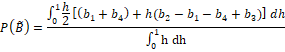
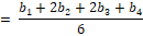
Graded mean Integration Representation Method was introduced by Hsieh et al 14 based on the integral value of graded mean h-level of generalized fuzzy number for the defuzzification of generalized fuzzy number. First, a generalized fuzzy number is defined as follows: Ã-=(α1, α2, α3, α4,)LR. By graded mean integration are the inverses of L and R are L-1 and R-1 respectively. The graded mean h-level value of the generalized fuzzy number Ã-=(α1, α2, α3, α4,)LR is given by h/2[L-1(h)+R-1(h)]. Then the graded mean integration representation of P(Ã) with grade then

In this paper trapezoidal fuzzy numbers is used as fuzzy parameters for the production inventory model. Let 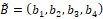 Then the graded mean integration representation is given by the formula as
Inventory Model For Eoq
The input parameters for the corresponding model are
K - Ordering cost
a - constant demand rate coefficient
b - price-dependent demand rate coefficient
P - selling price
Q - Order size
c - unit purchasing cost
g - constant holding cost coefficient
Let’s consider the total cost 15 and modify in a fuzzy environment
The total cost per cycle is given by
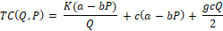
Partially differentiating w.r.t Q,
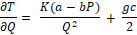
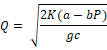
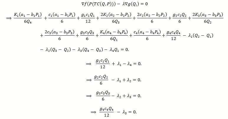
Equating  the economic order quantity in crisp values obtained as
Inventory Model For Fuzzy Order Quantity
By using trapezoidal numbers, fuzzified input parameters are as follows

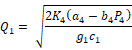
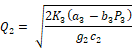
The optimal order quantity
Partially differentiating w.r.t ‘Q’ and equating to zero,

Hence the optimal economic order quantity for crisp values is derived,

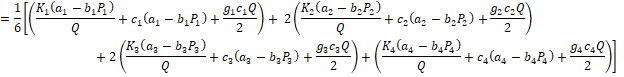
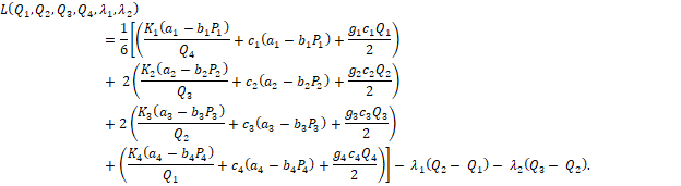
Applying the graded mean representation

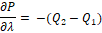
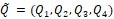
Now partially differentiating w.r.t Q1, Q2, Q3, Q4 and equating to zero,


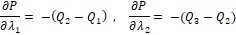
The above derived results depict that Q1 > Q2 > Q3 > Q4 failing to satisfy the constraints 0 ≤ Q1 ≤ Q2 ≤ Q3 ≤ Q4 . So, converting the inequality constraint Q2 - Q1 ≥ 0 into equality constraint Q2 - Q1 = 0 Optimizing P(TC(Q,P) subject to Q2 - Q1 = 0 by Lagrangian method.


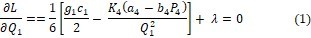
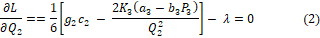


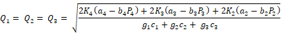
From equations (1) and (2) the results are,


Since Q3 > Q4 which does not satisfy the constraint 0 ≤ Q1 ≤ Q2 ≤ Q3 ≤ Q4. Now converting the inequality constraints Q2 - Q1 ≥ 0, Q3 - Q2 ≥ 0 into equality constraints Q2 - Q1 = 0 and Q3 - Q2 = 0. Optimizing,


From equations (1’) , (2’) and (3’),
In the above-mentioned results Since Q1 > Q4 which does not satisfy the constraint 0 ≤ Q1 ≤ Q2 ≤ Q3 ≤ Q4. Converting the inequality constraints Q2 - Q1 ≥ 0, Q3 - Q2 ≥ 0 and Q4 - Q3 ≥ 0 into equality constraints Q2 - Q1 = 0, Q3 - Q2 = 0 and Q4 - Q3 = 0 . Optimizing,

After Partially differentiation (Appendix)

satisfies the required inequality constraints.
Kuhn-Tucker Optimization Method
By applying Kuhn Tucker conditions, the total cost is minimized by finding the solution of Q1, Q2, Q3, Q4 with Q1, Q2, Q3, Q4

The above conditions simplify to the following 𝞴1, 𝞴2, 𝞴3, 𝞴4.
It is known that, Q1 > 0 then in

𝞴1Q1 = 0 arrive at 𝞴4 = 0 In a similar fashion, if 𝞴1= 𝞴2 = 𝞴3 = 0, Q4 ≤ Q3 ≤ Q2 ≤ Q1 does not satisfy 0 ≤ Q1 ≤ Q2 ≤ Q3 ≤ Q4. Therefore the conclusion is Q2 = Q1, Q3 = Q2 and Q4 = Q3
i.e., Q1 = Q2 = Q3 = Q4 = Q*
Numerical Examples
Let us consider an integrated inventory system having the following statistics with crisp parameters having following values 15, the ordering cost K=520 units, the optimal selling price P=36.52 units, unit purchasing cost c=4.75, g=0.2, constant demand rate coefficient a=100 units, price-dependent demand rate coefficient b=1.5.
As mentioned earlier, the trapezoidal numbers

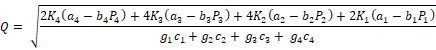
yielding the below results. Equation 1 was the optimal order quantity for crisp (equation 1) values and optimization to the EOQ is done by applying Lagrangian (equation 2) and Kuhn-Tucker (equation 3) methods under graded-mean defuzzification method. Figure 1 represents the crisp and fuzzified output varying on demand.
Figure 1. Variable demand for crisp and fuzzy comparison for EOQ
Conclusion
The fuzzified output varies at a larger rate than crisp output while varying the demand. This shows that the optimization results can be obtained only by restricting the controlling parameters. Figure 2 shows the variations in unit purchase cost for crisp and fuzzy output. An analysis of the total cost in a fuzzy environment is studied herewith by applying the Lagrangian and Kuhn-Tucker methods for optimization and using trapezoidal numbers. The value does not show much variation in optimal solutions. While varying the price-dependent demand rate coefficient among both the methods, fuzzified values decrease in Lagrangian and increases in the Kuhn-Tucker method. In Figure 3, the curves of crisp and fuzzy EOQ remain closer. Table 2 shows the comparison of graded mean values between the two optimization methods in operations research 13 Lagrangian and Kuhn-Tucker methods. The values are varied to an increase and decrease of 25% and 40% which clearly shows that the crisp values of EOQ stay perfectly aligned between both the methods. Figure 4 collates the three parameters viz., price dependent coefficient, purchase cost, and varying demand which shows the variations in 3D model. Table 1 & Table 2.
Figure 2. Variable demand for unit purchase cost for EOQ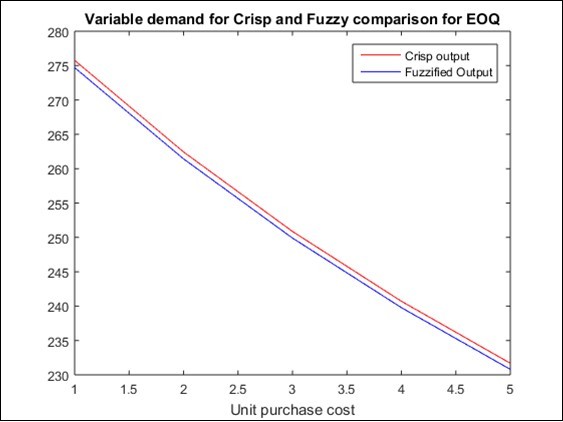
Figure 3. Variable demand for price dependent coefficient for EOQ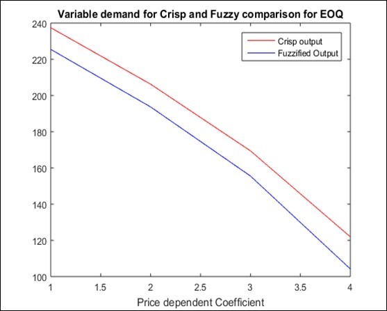
Figure 4. Three-dimensional variation of price dependent coefficient, demand and purchase cost.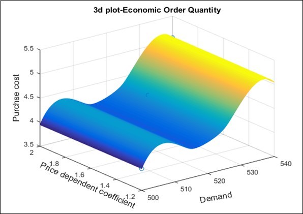
| Price-dependentco-efficient | Lagrangian method | Kuhn-Tucker method |
| b=1 | EOQ = 263.6169 | EOQ = 263.6169 |
| Fuzzy = 260.2202 | Fuzzy = 321.2251 | |
| b=1.5 | EOQ = 222.4949 | EOQ = 222.4949 |
| Fuzzy = 207.7356 | Fuzzy = 258.333 | |
| b=2 | EOQ = 171.7967 | EOQ = 171.7967 |
| Fuzzy = 147.1273 | Fuzzy = 194.5951 |
| Parameters | % change parameters | Graded-mean values | CrispEOQ | LagrangianMethod | Kuhn-Tucker Method |
| K(520) | +40% | 728(708,718,738,748) | 263.2595 | 246.140 | 305.902 |
| +25% | 650(630,640,660,670) | 248.7569 | 232.451 | 288.931 | |
| -25% | 390(370,380,400,410) | 192.6863 | 179.430 | 223.231 | |
| -40% | 312(292,302,322,332) | 172.3438 | 160.136 | 199.342 | |
| P(36.52) | +40% | 51.128(31.128,41.128,61.128,71.128) | 159.7376 | 106.502 | 128.4246 |
| +25% | 45.65(25.65,35.65,55.65,65.65) | 185.7729 | 147.128 | 178.9012 | |
| -25% | 27.39(7.39,17.39,37.39,47.39) | 253.9615 | 236.628 | 289.3353 | |
| -40% | 21.912(1.912,11.912,31.912,41.912) | 271.093 | 257.475 | 315.0044 | |
| a(100) | +40% | 140(120,130,150,160) | 305.4398 | 301.807 | 374.9838 |
| +25% | 125(105,115,135,145) | 277.2588 | 271.688 | 338.6781 | |
| -25% | 75(55,65,85,95) | 148.7803 | 127.422 | 168.3332 | |
| -40% | 60(40,50,70,80) | 75.5944 | 52.1485 | 49.2549 | |
| b(1.5) | +40% | 2.1(1.6,1.8,2.2,3) | 159.7376 | 134.7605 | 187.338 |
| +25% | 1.9(1.6,1.8,2,2.2) | 185.7729 | 180.8325 | 227.4581 | |
| -25% | 1.1(0.5,0.8,1.4,1.7) | 253.9615 | 250.2417 | 310.0121 | |
| -40% | 0.9(0.6,0.8,1,1.2) | 271.0938 | 271.8465 | 334.0561 | |
| c(4.75) | +40% | 6.7(6.4,6.5,6.9,7) | 188.0425 | 169.2837 | 210.5158 |
| +25% | 5.9(5.5,5.7,6,6.5) | 199.0055 | 179.1926 | 222.8382 | |
| -25% | 3.6(3,3.2,3.8,4.6) | 256.9150 | 223.8899 | 278.4223 | |
| -40% | 2.8(2.2,2.7,3,3.2) | 287.2397 | 258.3873 | 321.3222 | |
| g(0.2) | +40% | 0.28(0.18,0.2,0.3,0.5) | 188.0425 | 170.5264 | 212.0612 |
| +25% | 0.25(0.14,0.15,0.26,0.54) | 199.0055 | 176.1179 | 219.0145 | |
| -25% | 0.15(0.1,0.14,0.16,0.2) | 256.9150 | 241.4086 | 300.208 | |
| -40% | 0.12(0.1,0.11,0.13,0.14) | 287.2397 | 271.2692 | 337.3417 |