
CFD Simulation Study on Shell Made of Composite Material when Subject to Temperatures Above 3000 Degrees Centigrade
Abstract
In this article I am explaining the Computational Fluid Dynamics (CFD) simulation study on shell made of Composite material when subject to Temperatures above 3000ºC. In this analysis a shell is made of the composite structure with all the properties defines as of the Carbon Phenolic materials and is subjected to temperatures of 3000ºC and the flow pattern over the surface is studied and the velocity gradients on the shell when travelling with such high speeds and temperatures are studied. This simulation study can be used to predict the flow simulation in various applications of heat transmission. This CFD simulation study results are useful to make a CP composite material for better thermal applications in aerospace industry.
Article Information
- Received
- Accepted
- Published
Academic Editor: Mohammad Tavakkoli, Shahid Chamran University of Ahvaz, Ahvaz, Iran.
Checked for plagiarism: Yes
Review by: Single-blind
Copyright © 2020 C. Hari Venkateswara Rao, et al.
 This is an open-access article distributed under the terms of the Creative Commons Attribution License, which permits unrestricted use, distribution, and reproduction in any medium, provided the original author and source are credited.
Corresponding author: C. Hari Venkateswara Rao, Ph.D, Scholar, Mechanical, Engg, . Dept., UCE, Osmania University, Hyderabad – 07, Mobile: + —
Competing Interests
The authors have declared that no competing interests exist.
Funding
No specific funding statement was provided by the authors.
Data Availability
No data-availability statement was provided by the authors.
Citation:
Introduction
Composite materials are dominating all engineering materials and challenging for young engineers to know the characteristics about the composites in day to day life. The composite material are used into wide range of components to supply a diverse and fragmented commercial base that includes customers in aerospace, aircraft, defense, marine industry2. Phenolic composite products are commonly used in high temperature environment for relatively long period of time and light weight composition 3.
Composite materials are the most suitable materials for the design of aerospace structures like missile airframes, re-entry vehicle structures and air craft outer envelopes. Carbon-epoxy composites are used for mechanical strength bearing purpose and where as carbon-phenolic composites are used for thermal load bearing purpose in the missile structures. When re-entry of the vehicle takes place the temperatures they have to withstand are around 3000 degrees centigrade.
The major objective of this CFD simulation study is to made conical shell with properties of Carbon Phenolic (CP) and subjected to temperatures of 3000ºC to know the flow patterns over the surface of the shell and velocity gradients on the conical shell when travelling with high speeds and temperatures1 .
CFD Analysis
Grid Generation
The accuracy of prediction of flow behaviour strongly depends on its modelling to capture the exact flow phenomenon over the blade profile which requires a decent grid with optimum size of mesh or number of nodes. The mesh was generated in Ansys ICEM software tool for the required domain and the number of nodes initially is 10788.
Choosing Yplus
The y+ value is a non-dimensional distance from the wall to the first node of mesh (based on local cell fluid velocity) shown below. At low Re, for predicting the flow accurately, the mesh used should be so fine that can resolve the smallest turbulences or eddies in the flow.
As for present case low Reynolds number, it is important to place sufficient inflation layer cells to capture the flow behavior within laminar sub layer, a low value of y+=25 is desired 1. The distance of first node is estimated from the y+ calculator provided or from equation shown below. Figure 1.
Figure 1. Plot for determining the Y+ on the blade profile.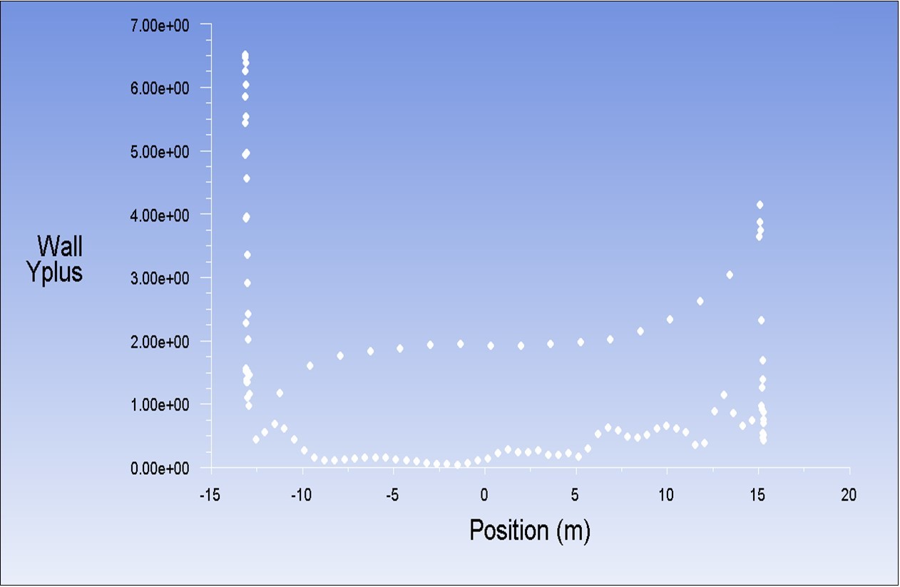
Download figure
Grid Verification
Grid Convergence
The mesh independence study was carried out by simulating with a selected numerical model for finer and finer meshes, considering two parameters CL. Figure 2.
Figure 2. Grid Convergence Graph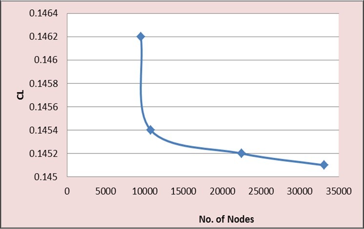
Download figure
Boundary Conditions
Inlet and Outlet Boundary Conditions
Velocity at an inlet and Static Pressure at an outlet as boundary conditions has been considered as the most robust conditions and was used for all the simulations.
Inlet velocity of 2000 m/s is set at Temperature of 3300K.
Shell wall motion taken as stationary wall and shear condition as No slip. The free stream temperature kept at 3300K with wall thickness of 0.025m. The density of material taken as 1850kg/m3 and Thermal conductivity as 202.4 w/m-k
Outlet gauge static pressure is set to zero.
Periodic boundary conditions are given to the outer wall and inner wall.
Turbulence Models Considered in FLUENT
In this present study the Reynolds-Averaged Navier-Stokes (RANS) approach only has been taken into account here because of its less computational demand. It involves in averaging the Navier-Stokes equations to get the term of Reynolds stresses. This alone cannot be solved directly and some additional equations are required to close the problem. The turbulence models role is to solve the additional equations. ANSYS Fluent contains several turbulence models, more or less they are complex, and they have been designed for different conditions and cases that are described below.
K-€ models
This model is based on two-equations, one is the transport equation for the turbulent kinetic energy (TKE) and other one is on turbulent dissipation rate (ϵ). Further, there are three sub models in ANSYS Fluent for the k-ϵ model.
Standard k-€
For industry purpose this model is very much popular and widely used. It is well known to be robust, reasonably accurate, and involves very low computational resources and time. It is being validated for especially high-Reynolds-number cases and large range of flows. However, it is not suitable in predicting flows with separation or swirl and large pressure gradients.
RNG k-€
RNG stands for “Re-Normalization Group theory”. This turbulence model is based on statistical technique and it is an advanced version of the standard model. The accuracy has been improved, as well as the ability of resolving swirling and low-Reynolds-number flows.
Realizable k-€
This turbulence model is used to solve exactly the spreading rate of coaxial and planar jets, flows comprising separation, rotation, recirculation or boundary layers involving robust adverse pressure gradients. The disadvantage of using this realizable model is that it can sometimes leads to a non-physical estimations of viscosities when the domain contains at the same time stationary and rotating regions.
K-ω models
This type of models are based on two equations like the one discussed earlier, one the transport of turbulent kinetic energy(k) and the other one specific dissipation rate (ω).
Standard k- ω
The Standard k-ω model is established on the one developed by Wilcox. It’s being designed to predict compressibility, low-Reynolds-number effects, and shear flow spreading. It is presently used in aerospace and turbomachinery industries.
SST k- ω
SST calls for Shear Stress Transport. The Standard k-ω and the k-ϵ are combined to put on the. The Standard k-ω turbulent model is utilised in the near wall region and the Standard k-ϵ model is utilised in the remaining domain. Thus this model is highly precise than the Standard k-ω and reliable for a extensive range of flows.
K-kl-ω Transition Model
This model is based on three equations, the additional equation when compared to the other two models is the modelling the laminar kinetic energy. This model has the capability to solve the development of the boundary layers and their transition from laminar state to turbulent state.
Transition SST Model
This is a four-equation model, which couples the model SST k-ω with two other transport equations, for transition beginning criteria. Similar to the k-kl-ω Transition model it also tries in predicting the transition of flow boundary layers.
Reynolds Stress Model (RSM)
The Reynolds Stress Model involves seven equations and is the most enlarged model existing in ANSYS Fluent, the transport equations of the Reynolds stresses are solved using this model The results obtained from this model are expected to be more accurate than the other models for complex flows. It is well used for high-anisotropic flows like cyclones, strong swirl in combustors etc.
Validation Method
The validation of the computational study is prepared by relating the obtained CFD results with experimental data and the CFD analysis carried out by Joshua R. Brinkerhoff, Harun Oria, and Metin I. Yaras. Hence it is fully depends on the experimental results available in the journal paper. Normally if the experimental results are not available then it is better to compare different turbulence models and the grid dependence test to be conducted to see how accurate the results obtained.
Koutmos and McGuirk used a new refined technique to create the flow-field within the lobe geometry. The method comprises of three basic steps. Firstly, the flow around the lobed mixer from the bypass and the core up to the exit plane of the lobe is determined. These exit conditions like the temperature fields and momentum are taken as inlet conditions to find the mixing duct flow area from the exit plane of the lobe and up to the outlet of the domain. Secondly, the coupling between all the three flows i.e. bypass, core and the mixing duct is established. The boundary conditions of the mixing duct in the downstream are used for recalculating the flow around the lobe mixer, mainly the at the inlet static pressure of the mixing duct. This let’s to catch the interaction between the bypass and core streams. The newly obtained exit conditions of the bypass and core flow are further used to re-predict the mixing duct flow. The criteria for convergence in this case is the relative changes of velocity and pressure fields at the outlet planes of the lobe and duct after each coupling phase.
Turbulence Models Considered in this Analysis
Equation Models
The recent 2 equation models are developed for solving the flow everywhere without using wall functions and hence k ω SST model is chosen to study for predicting the resulted flow phenomenon during the experiment.
k ω SST
This model solves for k; the turbulent kinetic energy, omega (ω) - the specific rate of dissipation of kinetic energy, combined with, the SST Shear Stress Transport (SST) model which is a combination of the k-epsilon in the free stream and the k-omega models near the walls. It does not use wall functions and tends to be most accurate when solving the flow near the wall. This model is used with Low Re & Curvature corrections. Figure 3.
Figure 3. Prediction of Turbulent Flow over a Sphere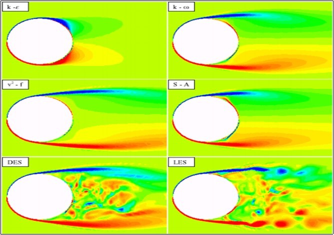
Download figure
Simulation Residuals
The figures below shows the residual captured during solution. All the residuals are reduced to less than or equal to 1x10⁻⁶ except the continuity and omega. Figure 4, Figure 5, Figure 6, Figure 7, Figure 8, Figure 9, Figure 10.
Figure 4. Residual recorded during the CFD simulation.
Download figure
Figure 5. Shows the contour of pressure variation over the shell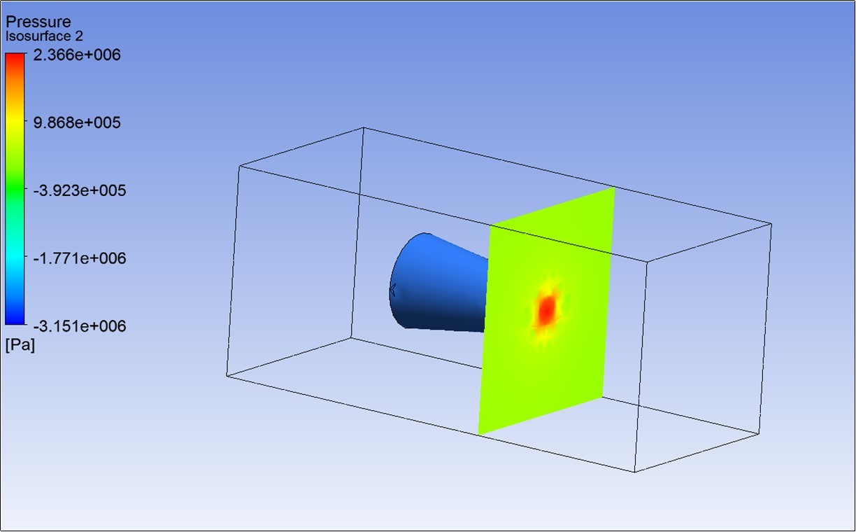
Download figure
Figure 6. Shows the contour of velocity variation over the shell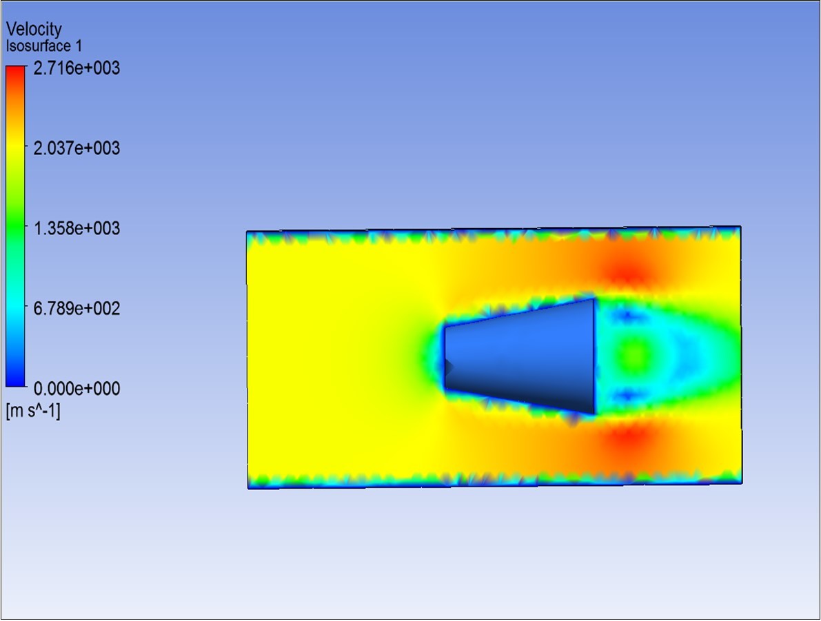
Download figure
Figure 7. Shows the contour of temperature variation over the shell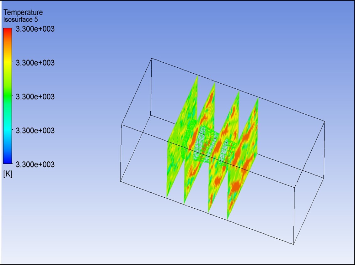
Download figure
Figure 8. Shows the contour of velocity vectors variation over the shell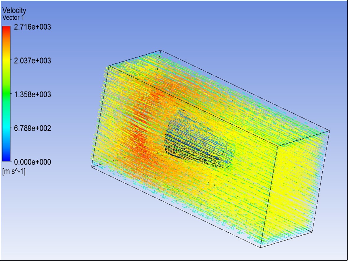
Download figure
Figure 9. Chart showing Pressure variation in the downstream in X direction over the shell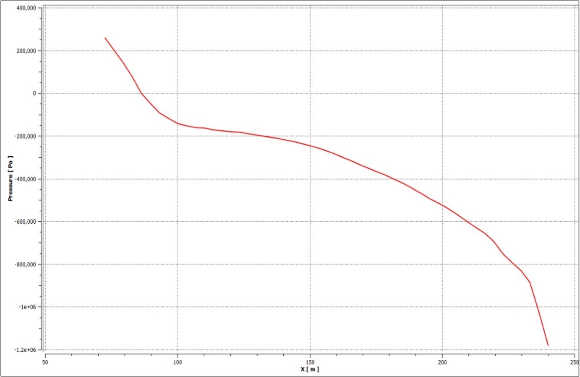
Download figure
Figure 10. Chart showing Velocity variation in the downstream in X direction over the shell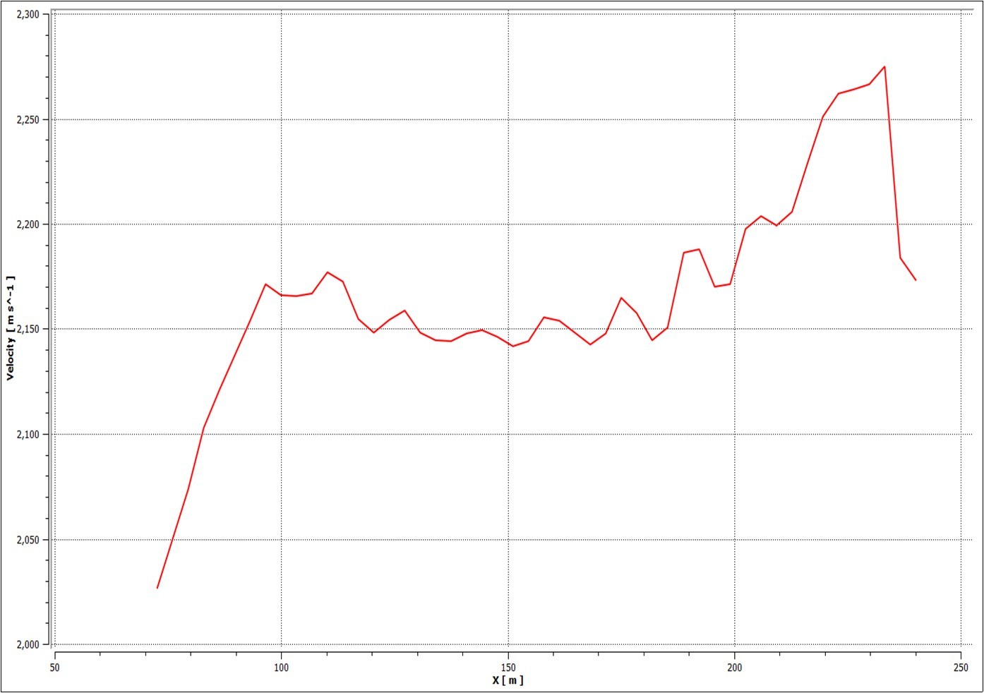
Download figure
Contour Plots
Conclusions
1. Firstly, from computational point of view, regarding the grid size it should be made with a good quality. Considering the complexity of the conical structures if it is very difficult to sustain the quality aspects of the structured grid an unstructured grid is good enough for this type of analysis. The computational time will probably be increase but more stable simulations are obtained.
2. Secondly, it is more accurate to use the pressure-based solver which is able to give right solutions and is good for compressible fluids. Also it reduces the computational time.
3. From Figure 8 it can be clearly seen that the velocity vectors when flown over the shell shows to be in turbulent in character and the same is observed in red color with velocity of 27160 m/sec.
4. It is observed clearly From Figure 6 the formation of boundary layer on the surface of the shell and the shear layer formation over the shell.
5. Figure10 shows that the velocity increased from 2175mm/sec to 2270mm/sec this shows that flow while passing over the shell boundary layer reaches turbulence as it passes the extreme side of the shell. There is a formation of wake at the end of the shell wherein the vortex formation is observed at the end. The same can be observed in Fig.6.
6. The pressure plot in Fig 9 shows that as the flow passes the shell region the pressures becomes negative which again shows the formation of wake region behind the shell.
7. CFD is an excellent tool to predict the flow simulation in various applications of fluid engineering systems using modelling and numerical methods.