Analysis of Covid-19 Using A Modified SEIR Model To Understand The Cases Registered in Singapore, Spain, And Venezuela
Abstract
This work proposes a modification of a compartmental-type model based on the Susceptible-Exposed-Infected-Recovered (SEIR) scheme to describe the dynamics of contagion by Covid-19 in any part of the world, including also the numerical and analytical calculation of the mantissa and the resolution of a partial differential equation system. As an example, the different incidents that occurred in Singapore, Spain and Venezuela are analyzed to demonstrate the usefulness of the methodology developed in this work that can be seamlessly extended to other regions.
Author Contributions
Copyright © 2022 Raúl Isea, et al.
 This is an open-access article distributed under the terms of the Creative Commons Attribution License, which permits unrestricted use, distribution, and reproduction in any medium, provided the original author and source are credited.
Competing interests
The authors have declared that no competing interests exist.
Citation:
Introduction
The world is facing a pandemic caused by Covid-19, which is caused by a SARS-CoV-2 betacoronavirus, after the first reported incidents in the city of Wuhan (China) in December 2019 in a wholesale seafood market. The pandemic has a record of more than 505 million Covid-19 infections and at least 6.2 million deaths until April 2022.
To date, cases have been registered in almost all the countries of the world, including Antarctica 1, where an incident at the Chilean research center located at the General Bernardo O'Higgins base on December 21, 2020 was notified. In fact, after examining the distribution of cases in the world, there is no uniform distribution; as an example, three different countries can be selected. The first is Singapore, where more than 1.16 million people have been infected with a population of 5.7 million inhabitants, despite the fact that 87.3% of the population has been vaccinated. The second case is Spain, where 11.6 million people have been infected with a population of 47.3 million inhabitants, 85.7% of which are vaccinated. Finally, in Venezuela, 522,055 cases have been registered among the 28 million inhabitants, where only 44.3% of the population has at least two doses of the vaccine.
These daily records of contagion in the world are compiled by various repositories due to health emergency worldwide, being one of those that from the Johns Hopkins Coronavirus Resource Center (freely available at https://coronavirus.jhu.edu/), as well as Our World in Data (https://ourworldindata.org/covid-cases), Worldometer (https://www.worldometers.info/coronavirus/), or the World Health Organization one (https://covid19.who.int/), among others.
Thanks to these daily records, public policies have been designed to contain this disease with the imposition of quarantines, social distancing measures, or the mandatory use of masks, among other measures 2, 3, 4. Despite this, outbreaks have emerged in the same country, which has not made it possible to contain this pandemic. As an example, we can cite the recent incidents in the city of Guangzhou, where restriction measures have been imposed again to stop the current outbreak, such as the closure of the city without allowing the landing of commercial flights.
To visualize the different epidemic outbreaks that have occurred in the countries, the mantissa calculations based solely on the daily registration of cases by Covid-19. The value of the mantissa runs from zero (no contagion) to one (no restrictions because of contagions), so it can be taken as an infection rate that is dependent on time 5, 6, 7.
To visualize this last paragraph, the corresponding mantissa for Singapore, Spain, and Venezuela are shown in Figure 1. The selection of these countries is random and the calculi can be applied to other countries and regions. This figure allows understanding, for example, that at the beginning of the outbreak, the virus was quickly expanding (oscillations in the mantissa value). Secondly, the duration of outbreaks increases over time in view of the different variants of Covid-19, with omicron being the most persistent in those countries, see details of the calculations in 5, 6, 7.
Because of the corona contagions, different mathematical model that could allow improving and controlling the different cases registered by Covid-19 were designed, regardless of the public policies implemented in any country in the world.
Figure 1.Calculation of the mantissa (orange) and the daily accumulated record of Covid-19 cases (blue) since the first recorded incident occurred in Singapore (top), Spain (middle), and Venezuela (bottom), where the diversity of infections that occurred in these countries can be seen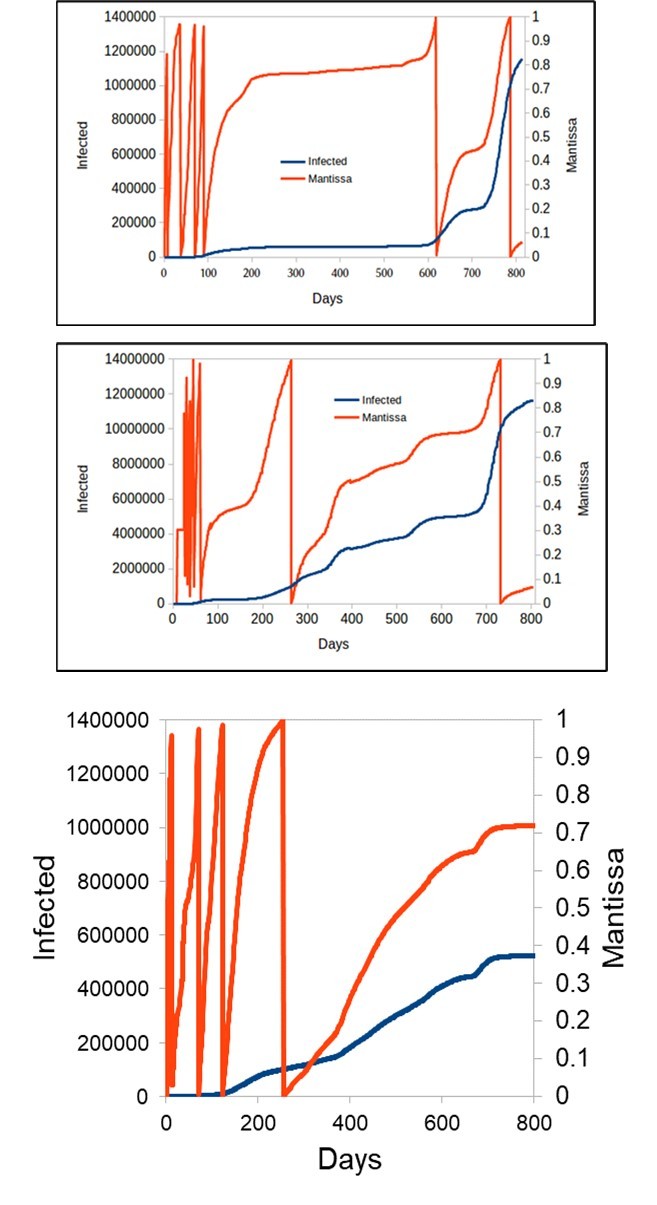
The most used model has been the compartimental one Susceptible-Infected-Recovered (SIR), which was introduced by Kermack, W. O., and A. G. McKendrick in 1927 8, and mathematical interpreted by Isea and Lonngren 9. This model is based on the fact that the entire population is susceptible (usually abbreviated as S) to contracting the Covid-19 virus. Later some people can be Infected (I) and finally people recover (R). It is important to clarify that this type of model does not discriminate between the infected population and that which is asymptomatic. Subsequently, a SEIR-type model was implemented, whose difference is that the population, before it is infected, is exposed to the virus (E). In fact, this type of model is a natural extension of the SIR model, whose first publication dates back to 1984 with the work published by Aron et al 10. In view of this, there is a large number of works that use the SEIR model to describe Covid-19, such as Chung and Chew 11 when explaining the spread in Singapore, as well as the work of Annas et al 12 when analyzing the cases that occurred in Indonesia.
In this model, the possibility of reinfection of people recovered from Covid-19 is not being considered, that is, the model assumes that recovered people have immunity and, therefore, cannot be reinfected. In view of the above, the present work develops and implements a variant of the Susceptible-Exposed-Infected-Recovered (SEIR) type model to explain the spread of Covid-19. This is intended to describe the contagion dynamics of this disease from the daily record of infected cases, so that it would be possible to predict the number of infected people per country in the short term.
Mathematical Model
Several models have been used to study the spread of the Covid-19 virus at a mathematical level. As an example, the recent work by Jayatilaka et al 13 uses three different models, of which two are based on the SIR/SIRmp model and one on the SEIR type variant. These authors conclude after analyzing their results: “The models discussed in this study have a good range of variability and applicability – but they are not perfect. It is important to note that these models assume ideal conditions so they may not truly reflect the true situation” 13.
So it is necessary to continue developing models that allow us to reproduce and, above all, predict the dynamics of virus spread. Likewise, the next step would be to calculate all the mathematical models and compare these results with the data recorded in the different countries and, even so, it would be difficult to ensure that we would be able to obtain a correct and valid model for all the countries in question since the exact number of infected people is unknown. All this, without taking into account social aspects such as social distancing measures, the degree of protection of the population that has been vaccinate 14.
In this sense, this work proposes a model based on a modification of the Susceptible-Exposed-Infected-Recovered (SEIR) model that has been recently introduced in the scientific literature 15 is used, where the population of a country (N) is split in the following parameters:
Susceptible, S(t), represents the entire population that is susceptible to contracting the disease
Exposed, E(t), is the proportion of people who are being exposed to the virus, but are not infected
Infected, I(t), corresponds to the case when people are infected by the virus, and finally
Recovered, R(t), are the people who have overcome the disease
This model is based on the following assumptions:
The population remains constant over time, so N is equal to S(t)+E(t)+I(t)+R(t)
There is a homogeneous mixture of the population and everyone gets sick in the same period of time
The population susceptible to contracting the disease decreases monotonically over time
There is no distinction between asymptomatically and symptomatically infected persons
The mortality rate is the same for all people, considering that the average age in the population is 60 years
There is no age distinction between people infected by Covid-19
All people are exposed to the virus, and there is no innate immunity
All people recover in the same time interval
The spread of the virus through the environment is not considered
Recovered people cannot be infected again by Covid-19
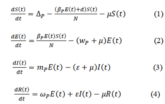
Figure 2 shows the scheme of the mathematical model used in this work ad sets the basis for analytically described the system, i.e., based on what was said above, the four differential equations that describe the dynamics of contagion by Covid-19 are then:
For simplicity and to be able to make a better adjustment of the parameters by the least squares method, it is normalized according to the total population of a country, so that the new expressions will be the following:
s(t) = S(t)/N,
e(t) = E(t)/N,
i(t) = I(t)/N,
r(t) = R(t)/N (5)
Since people cannot be infected again, it is possible to reduce the system to only three differential equations that will be described as follows:
Where Δp is the per-capita birth rate and also considers migration, so it is necessary to determine it by least squares. βp is the probability of disease transmission per contact and must be obtained for each country. μ is the per-capita natural death rate, which will be a set value for all countries, and equal to 0.01667. d is a global parameter on its own that considers the changes in the contagion rate of each country, and it must also be adjusted by a least squares method. mp is the infection rate obtained from the group of exposed people, while ε is the rate of change of the infected people (both constants must be determined by a least squares fitting). Finally, ωp is the rate of change of recovered people from exposed people (all these constants must be positive).
Taking into account the defined equations, the equilibrium points will be determined from the resolution of the system of equations, and later the parameters of the model are determined by a fitting of the parameters by a least squares method, which is the most used methodology to determine the different expressions of the mathematical model when real data are available.
Equilibrium Points
The procedure that has been described in the scientific literature to determine the equilibrium conditions based on the calculation of the critical or equilibrium points 16, 17, 18 is described below.
The equilibrium points are determined when the system of equations becomes equal to zero, that is:
A couple of equilibrium points are determined. The first equilibrium point, PC1, is determined when i=0, which corresponds to the case of a disease-free equilibrium, known as the disease-free point. By imposing this condition on equation we get that e=0 too. Using these values in equation (9), we obtain that

(12)
So the first PC1 is (Δp/d+μ ,0,0)
The second equilibrium point, PC2, is determined when i≠ 0, i.e., e ≠ 0, so it becomes (s*,e*,i*).
From Eq.11 is obtained that
And from Eq.10 it is deduced that
So applying the latest two results into Eq.9 it is obtained
i* = mpe*/(ε + μ)
Regrouping terms we reach
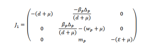
The next step is the calculation of the eigenvalues that will allow us to know the equilibrium conditions. Hence, it is necessary to calculate the Jacobian matrix (J) of the system of equations described by the system of equations (6-8), given by
Evaluating the Jacobian in PC1(denoted as J1) we obtain

Iterating this process for the second critical point ( J2) , we obtain
where J22 is defined by
It only remains to calculate the expressions of the eigenvalues (λ) to determine the equilibrium conditions of the system for each critical point. The eigenvalue evaluated for the first critical point (λ1) is obtained by the following expression of the eigenvalues
From this expression, the equilibrium point is reached when λ1 < 0 i.e., when (d+μ)(wp+μ)>βpΔp
And finally, two eigenvalues are obtained for PC2, an endemic system:
Least Squares Method
Lest squares fitting methodologies have been applied to different fields such as epidemiology, pharmacokinetics, biochemistry, radioactive isotopes, physiology and so on 19. Hence, variations have been designed as well, for example, Levenberg–Marquardt algorithm (LMA or just LM), also known as the damped least-squares (DLS) method 20. The latter is usually used to resolve linear least squares problems.
The calculation by a least squares method to determine the value of the parameters used in the mathematical model of this work is described in what follows. A function defined as ρ is minimized, which corresponds to the differences of the expressions of the values obtained from the function that is adjusted with respect to the observed values, which in this case are the daily record of the cases by the Covid-19. The function that is minimized is equal to:
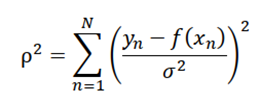
where n is the number of observed values to be fitted with the model. To do this, a program implemented in Python was designed to minimize the expression of ρ using the libraries developed in SCIPY 21. This algorithm has been used in other mathematical models that have been designed to understand the dynamics of contagion by Covid-19.
It only remains to note that a sensitivity analysis can be also performed in order to examine how the dependence of the parameters is after performing the least squares fitting, i.e. which parameters are the most sensible ones to the proposed model. Thus sensitive analysis has been performed via a very simple analysis based on the Morris Screening method was implemented using the ODEsensitivity library that is installed with R 22.
Results
Table 1 shows the different values of the parameters obtained from the system of differential equations (6-8) for Singapore, Spain, and Venezuela according to the records of the Johns Hopkins University. It is important to indicate that the final value obtained from the least squares fitting was 99.94%, 97.89%, and 84.41% for Singapore, Spain, and Venezuela, respectively.
After reading the values obtained in Table 1, we can roughly assume that: the values obtained from mp could indicate that the infection rate is similar in Venezuela and Singapore, unlike Spain, which has a higher value. However, the values obtained in wp, d, and mp reflect a similar behavior in the contagion dynamics between Spain and Singapore, different in Venezuela. In fact, Venezuela has a lower contagion rate (βp) compared to the other two countries.
As an example, the results obtained for Singapore are depicted in Figure 3. Green dots refer to the calculated ones, while orange dots are the observed ones. The advantage of obtaining the values of the parameters according to the registry of the cases is that it is possible to numerically determine the values of the critical points as well as the eigenvalues of the system in Table 2 and Table 3, respectively.
Table 1. Values obtained in the system of equations (6-8) for the targeted countries| Country | Population | β p | Δ p | m p | ε | d | w p |
|---|---|---|---|---|---|---|---|
| Singapore | 5453600 | 2.0754 | 0.7172 | 1.5481 | 0.0465 | 0.5611 | 2.4815 |
| Spain | 46745211 | 1.8036 | 0.8372 | 1.2068 | 0.0382 | 0.6212 | 2.277 |
| Venezuela | 28704947 | 1.5292 | 0.6791 | 1.5556 | 0.4342 | 1.181 | 0.844 |
| PC1 | PC2 | |||||
| Country | S* | E* | I* | S* | E* | I* |
| Singapore | 1.2411 | 0 | 0 | 1.2037 | 0.0087 | 0.1343 |
| Spain | 1.3126 | 0 | 0 | 1.2717 | 0.0113 | 0.2093 |
| Venezuela | 0.5669 | 0 | 0 | 0.5629 | 0.0057 | 0.0125 |
Table 3. Eigen values determined in each of the countries for PC2, where only one of the eigenvalues has been placed for the critical point 2.
| Country | λ1 | λ2 |
| Singapore | 0.0783 | (-0.5065, -0.0893) |
| Spain | 0.0742 | (-0.5770, -0.0813) |
| Venezuela | 0.0061 | (-1.2002, -0.0063) |
Figure 3.Results of the least squares method using the data from Singapore.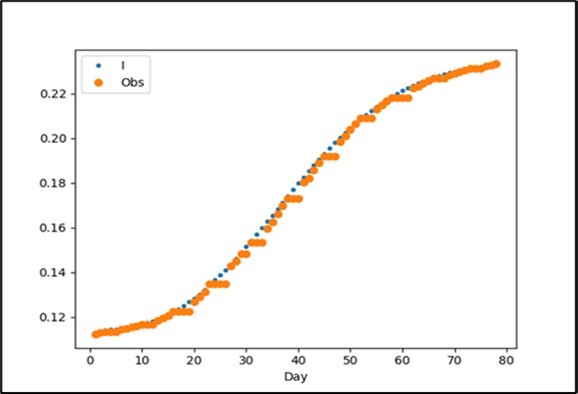
These three targeted countries present the same behavior as can be seen from Table 2 and Table 3, that is, the first equilibrium point is of the saddle point type, while the second is effectively an equilibrium point as it presents three negative values. Likewise, Venezuela presents a different behavior from the rest of the countries and among them, it is the one with the lowest number of infected cases since the beginning of the pandemic.
Finally, figure 4 shows the result of a sensibility analysis that indicates how the parameters depend on the mathematical model presented in the work. Important to remind that this is a preliminary calculation to highlight how sensitive the parameters obtained from the least squares adjustment are for each of the countries.
Figure 4.Sensitivity analysis results of the model presented in the work that describe the susceptible, exposed, and infected population; where βp, Δp, mp, ε , d, and wp, and are represented in yellow, red, sky blue (or light blue), purple, pink, and light green, respectively.
Conclusions
This paper presents a mathematical model based on the Susceptible-Exposed-Infected-Recovered model of the compartmental type for Covid-19. Three countries were selected whose behavior is completely different in the distribution of cases, and despite this, the adjustment of the data was quite good. The calculation of the mantissa also indicated the behavior of the continuous epidemic outbreaks in these countries, where the spread of the disease oscillated at the beginning and only after a 100-day period, the contagion rate started to decrease.
References
- 1.Frame B, A D Hemmings. (2020) Coronavirus at the end of the world:. Antarctica matters.Social Sciences & HumanitiesOpen 2(1), 100054.
- 2.Al-arydah M, Berhe H, Dib K, Madhu K. (2021) Mathematical modeling of the spred of the coronavirus under strict social restrictions.Math. Methods Appl. Sci. doi: 10.1002/mma.7965. Online ahead of print.
- 3.Bouchnita A, Checkroun A, Jebrane A. (2020) Mathematical modeling predicts that strict social distancing measures would be neede tos harten the duraction of waves. Covid-19 infections in Vietnam.Front PublicHealth 8, 559693.
- 4.Fang Y, Nie Y, Penny M. (2020) Transmission dynamics of the Covid-19 outbreak and effectiveness of government interventions: a data-driven analysis.J. , Med.Virol 92, 645-659.
- 5.Isea R. (2020) A new graph to display the epidemic outbreak. , of Covid-19 in the World.International Journal of Coronavirus 1(4), 1.
- 6.Isea R. (2020) A quick look at the registered cases of Covid-19 throughout the world.International. , Journal of Coronavirus 1(3), 15.
- 7.Isea R. (2022) What represent the mantissa of the registered. , Covid-19 cases.International Journal ofCoronavirus 3(2), 1.
- 8.W O Kermack, A G McKendrick. (1927) A contribution to the mathematical theory of epidemics.Proc. , R. Soc.Lond 115, 700-721.
- 9.Isea R, K E Lonngren. (2013) On the mathematical interpretation of epidemics by Kermack and McKendrick,General MathematicsNotes. 19(2), 83-87.
- 10.J L Aron, I B Schwartz. (1984) Seasonality and period-doubling bifurcations in an epidemic model.JTheorBiol. 110(4), 665-679.
- 11.Chung N N, Chew L Y. (2021) Modelling Singapore COVID-19 pandemic with a SEIR multiplex network model. , SciRep 11, 10122.
- 12.Annas S, M I Pratama, Rifandi M, Sanusi W, Side S. (2020) Stability analysis and numerical simulation of SEIR model for pandemic COVID-19 spread in Indonesia.Chaos Solitons Fractals. 139, 110072.
- 13.Jayatilaka R, Patel R, Brar M, Tang Y, N M Jisrawi. (2022) A mathematical model of COVID-19 transmission.Mater. , TodayProc 54, 101-112.
- 14.Lau H, Khosrawipour T, Kocbach P, Ichii H, Bania J. (2021) Evaluating the massive underreporting and undertesting of COVID-19 cases in multiple global epicenters.Pulmonology. 27(2), 110-115.
- 15.. HM Youssef, NA Alghamdi, MA Ezzat, AA Bary, AM Shawky. (2020). A modified SEIR model applied to the data of COVID-19 spread in Saudi Arabia editors-pick.AIPAdvances 10, 125210.
- 16.Isea R. (2013) Analysis of an SEIR-SEI four strain epidemic dengue model with primary and secondary infections.Revista Electrónica Conocimiento Libre yLicenciamiento. 7, 3.
- 17.Isea R, Mayo-Garcia R. (2015) Mathematical analysis of the spreading of a rumor among different subgroups of spreaders.Pure andAppliedmathematicalletters. 50-54.
- 18.Isea R. (2018) Analytical solutions for the initial steps of the intracellular dynamics of influenza a virus.Acta Scientific. , Microbiology 1(6), 6.
- 19.Bailer J, Portier C J. (1990) A note on fitting one-compartment models: Non-linear least squares versus linear least squares using transformed data.Journal of Applied Toxicology. 10(4), 303-306.
- 20.Pujol J. (2007) The solution of nonlinear inverse problems and the Levenberg-Marquardt method,Geophysics. 72(4), 1-16.

