
Abstract
Background
The relationship between predictors and the variable of interest was estimated using a structural equation model which is used to predict latent variables. The main advantage of the SEM is the ability to estimate the direct and indirect pathways of the effect of the primary independent variable on the outcome, given sufficient sample sizes. Despite not directly modeling the mediated pathways, GLMMs excluding mediating variables performed well with respect to power, bias and coverage probability in modeling the total effect of the primary independent variables on the outcome. In longitudinal studies, data are collected from subjects at several time points. The main purpose of longitudinal analysis is to detecting the trends or trajectories of the variables of interest.
Methods
A longitudinal study was conducted on 792 adults living with HIV/AIDS who commenced HAART. Structural equation modeling was used to construct a model to detecting predictors of CD4 cell count change. The procedure was illustrated by applying it to longitudinal health-related quality-of-life data on HIV/AIDS patients, collected from September 2008 to August 2012 monthly for the first six months and quarterly for remaining study period.
Results
The result of current investigation indicates that CD4 cell count change was highly influenced by certain socio-demographic and clinical variables. Out of all the participants, 141 (82%) have been considered 100% adherent to antiretroviral therapy. Structural equation modeling has confirmed the direct effect that personality (decision-making and tolerance of frustration) has on motives to behave, or act accordingly, which was in turn directly related to medication adherence behaviors. In addition, these behaviors have had a direct and significant effect on viral load, as well as an indirect effect on CD4 cell count. The final model demonstrates the congruence between theory and data (x2/df. = 1.480, goodness of fit index = 0.97, adjusted goodness of fit index = 0.94, comparative fit index = 0.98, root mean square error of approximation = 0.05), accounting for 55.7% of the variance.
Conclusions
The results of this study support our theoretical model as a conceptual framework for the prediction of medication adherence behaviors in persons living with HIV/AIDS. Implications for designing, implementing, and evaluating intervention programs based on the model are to be discussed.
Author Contributions
Academic Editor: Angela Pia Cazzolla, Department of Dentistry and Child Complex Operating Unit of Dentistry at the University of Bari
Checked for plagiarism: Yes
Review by: Single-blind
Copyright © 2020 Awoke Seyoum Tegegne
 This is an open-access article distributed under the terms of the Creative Commons Attribution License, which permits unrestricted use, distribution, and reproduction in any medium, provided the original author and source are credited.
Competing interests
The authors declare that they have n competing interests, which may have inappropriate influenced them in writing this article.
Citation:
Background
Longitudinal data is a core for researching exploration of changes of the various outcomes across a wide range of diesoline and different techniques are existed for analyzing such data 1. One of the approaches to study raw change scores which is computed as the deviation of outcomes/ values at time 1 and time 2 and these changes analyzed as a function of individual or group characteristics. The raw changes can be analyzed using t-test, ANOVA or multiple regression 2. An alternative to this , residual change scores can be computed as the residual between observed at time 2 and expected at time 2 results/values predicted by the time 1 values/ outcomes 3. Such changes are typically analyzed using multiple regression or analysis of covariance (ANCOVA) 4. Both raw and residualized change scores are useful for changes between two discrete time points analyzed in longitudinal prospective research designs 5. Both raw and residualized change scores are useful for changes between two discrete time points analyzed in longitudinal prospective research designs. Frequently, it is interesting to modeling developmental trajectories or patterns of changes in multiple time points and common approache to study such trajectories is to use standard growth analyses like repeated measures MANOVA or Structural Equation Modelling (SEM). Standard growth analyses estimate a single trajectory obtained by averaging from the individuals trajectories of participants 6. Structural equation modelling (SEM) consists of a system of simultaneous linear equations that describes relations among different variables 7. It also consists of non-linear equations those describe pattern of variance and covariance among variables. It includes Confirmatory Factor Analysis (CFA), Path Analysis (PA), Partial Least Square and Latent Growth Modelling (PLSLGM)8. These models are applied to evaluate unobservable (latent variables) and call upon an evaluation model that refers to latent variable applying one or more observable variables 9. Structural equation modeling has been developed mainly in the social and behavioral sciences. Structural equation modeling represents the complex relationships of variables as a sequence of linear equations. A prominent feature that distinguishes SEM from the more mainstream linear statistical modeling is the inclusion of latent factors in SEM. Previous researchers analyzed the longitudinal data that referred to as latent (growth) curve modeling (GCM) 10, 11. SEM is a power full mechanism that helps to combine complex path models with factors 12. It is a technique which assists to specify confirmatory factor analysis, regression models as well as complex path analysis. ML estimation for the constraints of particular structural equation with inadequate source of information can be applicable in SEM 13. Two stage least square estimator with its asymptotic distribution is inversely incorporated in SEM for the purpose of parameter estimation 14, 15. The link among the constructs of SEM may be approximate with self-determining regression equations or using advanced techniques. SEM has the ability to indicate associations among unobservable variables with manifest variables7, 16. SEM revealed mathematical parameter estimations (arrows) in the model with the extent of the associations. Further, to evaluate the theoretical constructs, it gives a chance to discover observable predictors that considerably expresses factors / latent variables. Researchers frequently use longitudinal data analysis to study the trends of health related issues 17. They might study how an elderly person’s CD4 cell count changes over time or how a therapeutic intervention affects a certain behavior over a period of time. Earlier contributions are found in the sociological and psychological literature 18, 19rather than modeling count or continuous response. The previous researches in SEM longitudinal data analysis mainly focused on main effects and not explored the interaction effects of covariates17, 19.
This paper introduces the structural equation modeling (SEM) approach to analyzing longitudinal data applying SEM. Basic interest in structural equation modelling is the conceptual constructs denoted by unobservable variables.The main advantage of the SEM is the ability to estimate the direct and indirect pathways of the effect of the primary independent variable on the outcome, given sufficient sample sizes. In longitudinal studies, data are collected from subjects at several time points. The SEM framework is a general modeling framework and allows the modeling of potentially complex relationships among observed and latent variables and can be applied in the longitudinal data setting. The main purpose of longitudinal analysis is to study the trends or trajectories of the variables of interest. For example, after a medical intervention, health measures might be taken every few months to monitor the health status of patients. Will their health improve, decline, or stay the same in the subsequent months or years? Do all the patients show the same health trajectory? The primary objective of the analysis is to evaluate the overall effect (main and interaction effect) of predictor variables on CD4 cell count.
Methods
Setting
We consider a longitudinal setting evaluating the impact of socio-economic and medial variables on CD4 cell count change on HIV disease progression. The data arise from a prospective cohort study in which the primary outcome, CD4 cell count change, is assessed monthly for the first six months and quarterly for the remaining study time (i.e. 23 measures of CD4 count across time for each subject), the time variate independent variables are also assessed at each follow-up visits. A potential mediator of the relationship between CD4 cell count change and potential predictors are associated with paths including with errors. In the current setting, HAART adherence is assessed at each of the follow-up visits. In addition to an indirect effect mediated by the lag variables (lag-1 and lag-2) variables, medical and socio-economic variables also have a direct biological effect on CD4 cell count. The study use real data that were collected in a study that looked at HIV/AIDS health related and the relationship between clinical and socio-economic variables and the variable of interest. Many different statistical approaches can be used to analyze this kind of data, including, but not limited to, SEM. Different fields have different traditions, and a particular field might favor one of these approaches or methodologies. This paper does not compare these approaches. Rather, it simply adopts the SEM approach to detect predictors using CALIS procedure in SAS and shows how several types of models are used for analyzing longitudinal data.
The Bayesian Estimates of Structural Equation Models
Let K be the arbitrary SEM with unidentified parameters β and let Y be the experimental data set of unrefined observed value with a sample size n. In Bayesian approach, β is random with a prior distribution and an associative /prior density function, say, p (β| K) 13, 20.
Let p (Y, β| K) be the possibility density function of the combined distribution of Y and β given K. The manner of β under the given data, Y is entirely explained by the conditional allocation of β given Y21. This conditional allocation is said to be the posterior distribution of β. Let p (β| Y, K) be the density function of the posterior distribution, based on the properties of density function in the probability theory, we have
p (Y’β| K) = p (Y|β, K) p(β)= p(β|Y, K) p(Y).
Since p(Y|K) is independent of β, and can be referred as constant with fixed Y, we have
log p (β|Y, N)α log p (Y|β,K) + log p(β) …..(1)
In (1), p (Y|β,K) can be considered as the likelihood function because it is the probability density of (y1, ….,yn) given the parameter vectorβ. The posterior density function in (1) indicates that it includes the sample information and the prior information through the likelihood function p(Y/β, K) and the prior density function P(β). In this condition, p (Y|β, K) is defined by the sample size, whereas p (β) is independent of the sample size. Hence, as a sample size becomes large, log (Y|βK) is closed to the log–likelihood function log P(Y|β, K). This indicates that Bayesian and ML techniques of estimation are approximately equivalent, and the Bayesian estimates have the same optimal properties as the ML estimates 22. However, the small or moderate sample size leads the prior distribution of β to play a significant role in the Bayesian approach. Accurate estimation can be obtained by including information in the analysis through the previous distribution of β. Thus, the selection of the prior density is an important issue in Bayesian analysis 23.
Former allocation of β indicates the distribution of probable values from which the parameter β has been selected. Prior distribution classified as informative and non-informative prior distributions. Non-informative prior distribution exists when the previous distribution has no population basis and sample distribution is used. Hence, the prior distributions play insignificant role in the development of posterior distribution 24.
A conjugate prior distribution is an example of usually used informative prior distribution in the general Bayesian approach in the analysis of statistical problems[25]. Let us consider the univariate binomial model expressed interims of β, the likelihood of an observed value y is of the form

Consider the prior density of β:
P (β)αβα-1 (1-β)θ-1 which is the beta distribution with hyper parameters α and θ. Then

Results
The baseline characteristics of study variables are indicated in Table 1.
Table 1. Baseline socio-demographic and clinical variables of 792 patients in the study| Variable | Average | No (%) | |
| Weight (kg) | 62 (58-70) | - | |
| Base line CD4 cells/ mm3 | 134 (113-180) | - | |
| Age (years) | 36 (28-48) | - | |
| First month / initial CD4 cell count change/mm3 | 15.9 (12-26) | - | |
| Sex | Male | 391 (49.4) | |
| Female | 401 (50.6) | ||
| Educational status | no education | 160 (20.2) | |
| Primary | 205 (25.9) | ||
| Secondary | 273 (34.5) | ||
| Tertiary | 154 (19.4) | ||
| Residence area | Urban | 468 (59.1) | |
| Rural | 324 (40.9) | ||
| Marital status | Living with partner | 355 (44.8) | |
| Living without Partner | 437 (55.2) | ||
| Level of income | Low income (< 500 ETB per month) | 355 (44.8) | |
| Middle income (5001-999 ETB per month) | 346 (43.7) | ||
| High income ( ≥ 1000ETB per month) | 91 (11.5) | ||
| WHO HIV stage | Stage I | 101 (12.8) | |
| Stage II | 258 (32.6) | ||
| Stage III | 199 (25.1) | ||
| Stage IV | 234 (29.5) | ||
| Disclosure | Yes | 575 (72.6) | |
| No | 217 (27.4) | ||
| Cell ownership | yes | 400 (50.5) | |
| No | 392 (49.5) | ||
| First monthHAART adherence | Good | 540 (68.2) | |
| Fair | 160 (20.2) | ||
| Poor | 92 (11.6) | ||
As shown in Table 1, out of the sample of 792 patients, 40.9 % were rural residents, 50.6 % were females, 44.8 % were living with their partner, 72.6 % disclosed their disease to family members, and 50.5 % were owners of cell phones. Lastly, 68.2% of the patients had good adherence and the rest were non-adherent (Fair +Poor) patients. Few of patients (11.5%) were high income level and 20% of them had no education.
Model fitting for CD4 cell count data using structural equation modelling
One means of assessing the determinants of the change of CD4 cell count is Structural Equation Modelling (SEM). Considering the commonly significant covariates on the variable of interest on the previous chapters, let us apply structural equation modelling to see whether or not the significant variables found above are also significant in this case. In our case, all dependent and independent variables are manifest/observable variables. Let rectangles in Figure 1 represent the manifest variable and circles for errors that can be created during estimation of parameters26.
Considering the current change of CD4 cell count as endogenous variable, the predictor variables (HAART adherence, weight, age, baseline CD4 cell count, visiting time and Cell phone ownership) found as significant variables from the previous chapters can be considered as exogenous variables. Since CD4 cell count results from the two previous results (prior one unit from the current and prior two units from the current) in transition model were significant for the current change, they had been included as predictor variables. Consider the first two lag variables (lag-2 and lag-1) as exogenous variable as shown in Figure 127.
Figure 1.Single factor measurement model for CD4 cell count change for adult HIV patients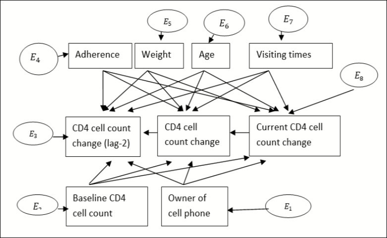
In Figure 1, the change in current CD4 cell count at lag-2, CD4 cell count change at lag-1 and current CD4 cell count change were considered as endogenous variables whereas ownership of cell phone, baseline CD4 cell count, adherence, weight, age and visiting times were considered as exogenous variables. 01, 02, 03 are observed linkages with adherence to their endogenous variables (CD4 cell count change for lag-2, lag-1 and current CD4 cell count change) and 04, 05 , and 06 are linkages with weight to its endogenous variables. Similarly, let 07, 08 and 09 be linkages from age, 010, 011 and 012 be linkage with visiting times, 013 013, 014 and 015 are linkages with initial CD4 cell count and 016, 017 and 018 are linkages from ownership of cell phone. (Table 2)
Table 2. Tests of goodness- of- fit for saturated and null models| RMSEA model | GFI model | |||||||
| RMSEA | 95 % C.I | P-value | RMR | GFI | AGFI | PGFI | ||
| Saturated model | 0.0320 | -0.0002 | 0.0653 | 0.7820 | 0.0805 | 0.9973 | 0.9855 | |
| Null model | 0.2970 | 0.3769 | 0.4047 | 0.0001 | 4.2453 | 0.4821 | 0.2896 | 0.4353 |
The goodness-of-fit statistic is indicated in Table 1. The chi-square test statistics is not significant at 0.05 which indicates that the model is good and accepted28. The root mean square error approximation (RMSEA) was 0.00334 that is less than 0.05. The goodness-of-fit index (GFI) and adjusted goodness-of-fit index were 0.9973 and 0.9855 respectively. Such results indicate that the model was good to fit the data at 95% CI and gave, X215= 9.96, P-value = 0.09843.
From Table 2 (RMSEA model), the p-value for default model is 0.7820 which indicates that there is no evidence for rejection of the null hypothesis that states the model is good. So, we have to choose the saturated model rather than the null model. (Table 3 and Table 4)
Table 3. Standardized regression weights for default model| Estimate | |
| Current CD4 cell count change <------------ CD4 cell count change (lag-2) | 0.62463 |
| Current CD4 cell count change <------------ CD4 cell count change (lag-1) | 0.21497 |
| Current CD4 cell count change <------------------------------------ adherence | 0.56231 |
| Current CD4 cell count change <-----------------------------------------weight | 0.22354 |
| Current CD4 cell count change <---------------------------------------------- age | 0.83452 |
| Current CD4 cell count change <-----------------------baseline CD4 cell count | 0.35463 |
| Current CD4 cell count change <-------------------------------------Visiting times | 0.21487 |
| Measurement | coefficient | S.E | Z | P-value | 95% C.I | |
| Adherence <------- CD4 count change | 1(const.) | |||||
| Constant | 96.31 | 1.38 | 74.5 | <0.001 | 92.79 | 98.77 |
| Weight <------ CD4 count change | 3.27 | 0.12 | 9.7 | <0.001 | 1.95 | 5.52 |
| Constant | 97.08 | 1.47 | 72.6 | <0.001 | 94.42 | 102.44 |
| Age <------ CD4 count change | 4.03 | 0.13 | 8.91 | <0.001 | 1.81 | 7.45 |
| Constant | 97.10 | 1.35 | 71.6 | <0.001 | 94.44 | 99.76 |
| Baseline CD4count <------CD4 count change | 1.05 | 0.61 | 11.42 | <0.001 | 0.08 | 3.98 |
| Constant | 45.77 | 5.88 | 75.43 | <0.001 | 26.34 | 64.44 |
| Visiting time <------CD4 count change | 1.02 | 0.51 | 10.42 | <0.001 | 0.01 | 2.89 |
| Constant | 60.77 | 5.88 | 97.43 | <0.001 | 36.34 | 74.43 |
| Owner of phone <------CD4 count change | 1.24 | 0.61 | 11.42 | <0.001 | 0.07 | 3.98 |
| Constant | 36.76 | 4.85 | 94.43 | <0.001 | 22.34 | 92.43 |
| Lag-2 <------CD4 count change | 1.14 | 0.54 | 34.32 | 0.012 | 0.02 | 3.35 |
| Constant | 32.38 | 4.68 | 65.32 | 0.003 | 28.76 | 42.53 |
| Lag-1 <------ CD4 count change | 1.07 | 0.84 | 43.42 | 0.012 | 0.01 | 4.45 |
| Constant | 35.48 | 5.58 | 68.52 | 0.003 | 26.76 | 45.43 |
| Variance of E *weight | 53.47 | 1.92 | 37.15 | 76.17 | ||
| Variance of E *age | 34.25 | 9.81 | 23..36 | 58.33 | ||
| Variance of E* visiting times | 96.15 | 67.62 | 54.84 | 98.61 | ||
| Variance of CD4 cell count | 18.20 | 24.32 | 12.43 | 27.46 | ||
(Table 5) indicated that current CD4 cell count change increased as adherence increased. Similarly, CD4 cell count change at these stages increased for patients having cell phone. In addition to predictors to CD4 cell count change, the previous two responses (CD4 cell count change at lag2 and lag1) had significant effect on the current CD4 cell count results. The expected log of CD4 cell count change increased as level of adherence increased. Likewise, for one unit increase of the expected log of CD4 cell count change at lag-2, the expected log of the current CD4 cell count change increased by 0.24 cells per mm3, keeping the others constant.
Table 5. Parameter estimation for saturated model in structural equation modelling| Estimate | S.E | C.R | P-value | |
| Adherence <--------CD4 cell count change at lag2 | 0.6546 | 0.0568 | 10.0462 | *** |
| Adherence<-------- CD4 cell count change at lag1 | 0.22497 | 0.0551 | 4.0839 | *** |
| Adherence <--------- current CD4 cell count change | 0.28497 | 0.0451 | 4.0839 | *** |
| weight <------------- CD4 cell count change at lag2 | 0.58916 | 0.0558 | 10.5581 | *** |
| weight <------------- CD4 cell count change at lag1 | 0.38916 | 0.0458 | 8.5581 | *** |
| weight <-------------- current CD4 cell count change | 0.38916 | 0.0458 | 8.5581 | 0.2312 |
| Age <------------------ CD4 cell count change at lag2 | 0.24762 | 0.0453 | 6.4352 | *** |
| Age <------------------ CD4 cell count change at lag1 | 0.83452 | 0.0874 | 6.3542 | *** |
| Age <------------------ Current CD4 cell count change | 0.65483 | 0.4563 | 4.5433 | *** |
| Initial CD4<----------- CD4 cell count change at lag2 | 0.65463 | 0.0568 | 10.0462 | *** |
| Initial CD4<------------ CD4 cell count change at lag1 | 0.22487 | 0.0551 | 4.0839 | *** |
| Initial CD4<---------- Current CD4 cell count change | 0.58916 | 0.0558 | 10.5581 | *** |
| Owner of Cell phone<---- CD4 cell count change at lag2 | 0.65326 | 0.0568 | 1.0462 | *** |
| Owner of Cell phone <-- CD4 cell count change at lag1 | 0.23497 | 0.0551 | 4.0839 | *** |
| Owner of Cell phone <-- Current CD4 cell count change | 0.67916 | 0.0558 | 12.5581 | *** |
| CD4 count(lag-2) <------ CD4 cell count change (lag-1) | 0.56326 | 0.05682 | 1.04618 | *** |
| CD4 count(lag-1) <----- current CD4 cell count change | 0.32497 | 0.15409 | 4.06390 | *** |
| Covariance for saturated model | ||||
| E1<------->E4 | 1.45324 | 0.34524 | 4.65421 | *** |
| E6<------->E7 | 0.65224 | 0.64824 | 4.65421 | 0.08532 |
| E2<------->E3 | 0.64327 | .65482 | 3.12537 | *** |
| E6<------->E7 | 0.75412 | .06831 | 2.3451 | 0.32130 |
| E3<------->E8 | 0.82453 | .67543 | 3.45632 | *** |
| E3<------->E5 | 1.43271 | .86541 | 2.54321 | *** |
| E5<------->E6 | 0.94231 | .32107 | 0.97421 | 0.32172 |
| E2<------->E8 | 1.63261 | .85321 | 2.54511 | *** |
| E1<------->E2 | 0.68261 | .95321 | 0.84511 | 0.14522 |
| E4<------->E8 | 0.98212 | .54132 | 3.42152 | *** |
| E7<------->E8 | 1.34252 | 1.22412 | 2.53214 | *** |
| E4<------->E5 | 0.86521 | .86241 | 1.86912 | 0.08321 |
| E6<------->E8 | -0.86312 | .94321 | 1.86321 | *** |
The correlation structure between E1<--->E4, E2<--->E3, E3<--->E5, E2<--->E8, E6<--->E8, E4<--->E8, E7<--->E8 and E3<--->E8 had significant effect on the relationship between endogenous and exogenous variables. In order to assess estimated value of linkage for each covariate on CD4 cell count change, standardized regression weights and the structural equation model are needed.
Discussion
In current investigation, the structural equation models for analysis of longitudinal data on univariate models of observable variables (CD4 cell count change) that are conditional to the other variables (time-varying or time invariant) were reviewed. Hence, in the paper keeping the statistical theory to be a practical guide for analysing longitudinal data, SEM applied for analysis of longitudinal data(CD4 cell count change and its predictors). However, considering the readers’ concept and prior knowledge of SEM, the investigators largely avoid dwelling on the basis of SEM. Although common software packages such as SAS and R have the capability to run SEMs, software designed specifically for SEMs 22 may be more intuitive and user-friendly in model specification, particularly in the development of highly complex models.
The current study examines one specific setting of mediated longitudinal data. Other situations with different data structures where mediation is present could also be explored, e.g. situations where the mediator and the primary independent variable as well as the outcome are repeatedly measured, categorical outcomes, and settings with more complex pathways between variables. In addition, we specifically explored the question of whether the LMM performs sufficiently in a setting favorable to the SEM. Future studies examining broader settings where the data arise from non-SEMs would provide further insight into the use of the LMM and SEM in mediated longitudinal settings. First, we found the factor loadings and intercepts of HD (health distress) and EF (energy and fatigue) not to be invariant across measurement occasions and, second, we found direct effects of CD4-cell count on EF and RF (role-functioning)29. The first two findings of measurement bias are considered as response shift by definition, as the measurement invariance is violated by the time of the measurement occasion. However, upon inspecting the HD and EF parameter estimates (Table 2) there did not appear to be an obvious substantive explanation for the changes in the factor loadings of HD. The other two findings of measurement bias are considered as response shift only if they vary with time. The bias in EF with respect to CD4-cell count is consistent over time and therefore not considered as response shift 30. The bias in RF with respect to CD4-cell count did vary with time, but again, it was difficult to provide a substantive explanation for this so-called response shift 31. Perhaps some of our results are chance findings, despite our best attempts to guard against such findings.
The Bonferroni adjustment of the level of significance guards against inflation of the family-wise error rate, but the chi-square difference test can still be affected by model complexity and sample size 32. In a simulation study, Cheung and Rensvold (2002) considered various alternatives to the chi-square difference test for testing across group constraints in multi-group factor analysis, and recommended inspection of differences in Bentler’s (1990) comparative fit index (among others). In our longitudinal factor analysis, we complemented the chi-square ifferences with ECVI differences, really only in order to provide additional information about the necessity of further modifications that cannot be substantively justified. In the present analyses, the ECVI differences generally agreed with the chi-square difference tests at Bonferroni adjusted levels of significance. One notable exception was that according to the 90% confidence interval of the ECVI difference, the fit of Models 2.2 and 2F was essentially equivalent, suggesting that constraints on EF factor loadings and intercepts could have been retained.
It should be noted that most response shift researchers in substantive areas of psychology contend that response shifts are the result of some catalyst event, such as an intervention in educational research (Howard et al. 1979), or a health state change in medical research (Sprangers and Schwartz 1999). In the HRQL study of HIV/AIDS patients, there is not a well defined event that all respondents have in common, other than having been diagnosed with HIV or AIDS some time ago. However, the time since diagnosis and the time on HAART vary greatly across patients and cannot be considered true catalysts. The one thing all patients have in common is that they participate in the HRQL study, and that they complete HRQL tests every half year. The test taking itself can have an effect on their response behaviour, which may change with time. The patients may become more accustomed to both their disease and taking the test, which perhaps induces a response shift. It should also be noted that most work on response shift in substantive psychological research was not aimed at investigating measurement invariance, but rather at explaining paradoxical intervention effects. Seeing that research into response shift was hampered by researchers having different conceptions of response shift, Oort (2005b) proposed to formally define response shift as a special case of measurement bias, although some researchers may still have another perspective on response shift (Oort et al. 2009).
As is illustrated by the empirical example, Step 2 and Step 3 of the detection procedure are laborious and time consuming. Especially if the numbers of observed variables and exogenous variables are large, these two steps involve the fitting of numerous models, in order to evaluate the chi-difference tests. An advantage of using modification indices is that, within each iteration, the researcher only has to fit a single model. Therefore, although perhaps less sound (Kaplan 1990), we explored the use of the modification index as an alternative to the global tests with multiple degrees of freedom.
When we evaluated the modification indices with the Bonferroni adjusted levels of significance, none of the findings were significant because of the large number of tests under consideration (e.g. 120 in Step 2). When testing at less conservative levels of significance, for example by considering tests of intercept constraints first and factor loading constraints second, or by simply raising the family-wise level of significance, there was a number of modification indices that reached significance.
However, as multiple modification indices were about equally large, the choice of which constraint to remove first seemed arbitrary, yet highly consequential for the removal of constraints in subsequent iterations, leading to very different conclusions. In addition, we also had to be careful not to run into constraint interactions. Still, the most important problem with relying on modification indices and less conservative testing was that many of the modifications were difficult to interpret and that the number of iterations grew very large. Saris et al. (2009) suggest only modifying models if the modification indices are associated either with moderate (instead of high) statistical power or with substantial expected parameter changes. When statistical power is high, one can only rely on substantive arguments for modification (ibidem), which we did, as in the present analyses the power to find medium sized differences was consistently above 99%.
In such situations, the decision making becomes increasingly subjective, as researchers will have to base their decisions between modifications and when to stop modifications on the interpretability of the different modifications. It is therefore highly likely that different researchers, with different substantive knowledge and different interpretation skills, will end up with different conclusions when analysing the same data. As can be seen from the procedure using modification indices, subjectivity in measurement bias detection influences whether and where bias is found. Notall researchers may want to test every possible combination of tenable equality constraints.
When this is the case, a priori hypotheses driven by theory should be stated before analysis and only these tests should be conducted. Under these circumstances, chance findings may further be reduced and more generalisable results found.
The problems associated with devising an objective procedure for measurement bias detection is common to specification searches in general. Bollen (2000): “Modelling strategies are subject to debate for virtually all statistical procedures. Witness the sharp disagreements over stepwise regression, the interpretation of clusters in cluster analysis, or the identification of outliers and influential points. The largely objective basis of statistical algorithms does not remove the need for human judgment in their implementation.” Similarly, when investigating measurement invariance, it is impossible to completely remove the element of human judgement. This is certainly true for the substantive interpretation of apparent measurement bias. However, we think that the procedure presented in this paper, with its safeguards against chance findings, at least helps to more objectively decide which measurements are biased and which are not.
Ethical Consideration
Ethical clearance certificate had been obtained from two universities namely Bahir Dar University, Ethiopia with Ref ≠ RCS/1412/2006 and University of South Africa (UNISA), South Africa, Ref ≠ : 2015-ssr-ERC_006 . We can attach the ethical clearances certificate up on request.
Consent for Publication
This manuscript has not been published elsewhere and is not under consideration by another journal.
Availability of Data and Materials
The secondary data used for current investigation is available with the corresponding author.
Funding
Not applicable
Acknowledgements
Amhara Region Health research & laboratory Center at Felege-Hiwot Referral Hospital, Ethiopia is gratefully acknowledged for the data supplied in our health research.
References
- 1.Singer J, Willet J. (2003) A framework for investigating change over time. Applied longitudinal data analysis: Modeling change and event occurrence. 3-15.
- 2.Alessandri G, Zuffianò A, Perinelli E. (2017) Evaluating Intervention Programs with a Pretest-Posttest Design: A Structural Equation Modeling Approach. Frontiers in Psychology. 8.
- 3.T M Achenbach.Future directions for clinical research, services, and training: evidence-based assessment across informants, cultures, and dimensional hierarchies. , Journal of Clinical Child & Adolescent Psychology 46(1), 159-169.
- 4.Bishop J, Geiser C, D A Cole. (2015) Modeling latent growth with multiple indicators: A comparison of three approaches. Psychological methods. 20(1), 43.
- 5.Isiordia M, Ferrer E. (2016) Curve of Factors Model: A Latent Growth Modeling Approach for Educational Research. Educational and Psychological Measurement. 0013164416677143.
- 6.Jung T, Wickrama K. (2008) An introduction to latent class growth analysis and growth mixture modeling. Social and personality psychology compass. 2(1), 302-317.
- 7.King-Kallimanis B, Oort F, Garst G. (2010) Using structural equation modelling to detect measurement bias and response shift in longitudinal data. AStA Advances in Statistical Analysis. 94(2), 139-156.
- 8.Barendse M, Oort F, Garst G. (2010) Using restricted factor analysis with latent moderated structures to detect uniform and nonuniform measurement bias; a simulation study. AStA Advances in Statistical Analysis. 94(2), 117-127.
- 9.Paldus J, Čížek J, Shavitt I. (1972) Correlation Problems in Atomic and Molecular Systems. IV. Extended Coupled-Pair Many-Electron Theory and Its Application to the B H 3 Molecule. Physical Review A 5(1), 50.
- 10.K A Bollen, P J Curran. (2006) Latent curve models: A structural equation perspective.John Wiley & Sons.Vol. 467.
- 12.K J Preacher, A F Hayes. (2008) Asymptotic and resampling strategies for assessing and comparing indirect effects in multiple mediator models. Behavior research methods. 40(3), 879-891.
- 13.Pástor Ľ, Sinha M, Swaminathan B. (2008) Estimating the intertemporal risk–return tradeoff using the implied cost of capital. , The Journal of Finance 63(6), 2859-2897.
- 14.Solomon S D. (2005) Cardiovascular risk associated with celecoxib in a clinical trial for colorectal adenoma prevention. , New England Journal of Medicine 352(11), 1071-1080.
- 15.Farebrother R W. (1999) Fitting Linear Relationships: A History of the Calculus of Observations.SpringerScience&BusinessMedia.1750-1900.
- 16.Davis C S. (2002) Statistical methods for the analysis of repeated measurements:Springer Science&Business Media.
- 17.R C MacCallum, Lee T, M W Browne. (2012) Fungible parameter estimates in latent curve models. Current topics in the theory and application of latent variable models. 183-197.
- 18.Yung Y, Zhang W. (2011) Making use of incomplete observations in the analysis of structural equation models: The CALIS procedure's full information maximum likelihood method. in SAS/STAT® 9.3. in Proceedings of the SAS® Global Forum 2011 Conference. SAS Institute Inc , Cary, NC .
- 19.K A Bollen. (2002) Latent variables in psychology and the social sciences. Annual review of psychology. 53(1), 605-634.
- 21.Palomo J, Dunson D B, Bollen K. (2007) Bayesian structural equation modeling. Handbook of latent variable and related models. 1, 163-188.
- 23.A E Raftery. (1996) Approximate Bayes factors and accounting for model uncertainty in generalised linear models. Biometrika. 83(2), 251-266.
- 25.Kline R B. (2015) Principles and practice of structural equation modeling. Guilford publications.
- 26.Bryan A, S J, M R Broaddus. (2007) Mediational analysis in HIV/AIDS research: Estimating multivariate path analytic models in a structural equation modeling framework. AIDS and Behavior. 11(3), 365-383.
- 27.Rosel J, Plewis I. (2008) Longitudinal data analysis with structural equations. Methodology. 4(1), 37-50.
- 29.Friis-Møller N. (2003) Cardiovascular disease risk factors in HIV patients–association with antiretroviral therapy. Results from the DAD study. Aids. 17(8), 1179-1193.
- 30.A N Phillips. (2001) HIV viral load response to antiretroviral therapy according to the baseline CD4 cell count and viral. 286(20), 2560-2567.