
Abstract
The isohydricity conditions are formulated for D+T systems composed of titrand D and titrant T, mixed according to titrimetric mode; only acid-base equilibria are involved there. The original method of dissociation constants determination, based on the isohydricity principle, is presented and confirmed experimentally. The pH titrations in the system of isohydric solutions are also put in context with conductometric titrations.
Author Contributions
Academic Editor: Zhe-Sheng Chenz, Professor, Department of Pharmaceutical Sciences, College of Pharmacy and Allied Health Professions, St. John’s University, United States.
Checked for plagiarism: Yes
Review by: Single-blind
Copyright © 2020 Anna M. Michałowska-Kaczmarczyk, et al.
 This is an open-access article distributed under the terms of the Creative Commons Attribution License, which permits unrestricted use, distribution, and reproduction in any medium, provided the original author and source are credited.
Competing interests
The authors have declared that no competing interests exist.
Citation:
Introduction
Titrimetric methods of analysis are commonly involved with mixing the solutions of two substances endowed with opposite properties, e.g., acid with base (B ⇨ A), or vice versa (A ⇨ B) 1, 2. Mixing two different acids (A1 ⇨ A2) or two bases (B1 ⇨ B2) according to titrimetric mode is usually not practiced. However, the special, isohydricity property is attributed here to solutions of two different acids, A1 and A2, or two different bases, B1 and B2, having equal pH values, i.e., the term “isohydric” refers to solutions of the same hydrogen-ion concentration, [H+1]. After Arrhenius, such a pair of solutions is termed as isohydric solutions 3, 4.
However, the Arrhenius’ statement 5, expressed in more contemporary terms, as “if two solutions of the same pH are mixed, pH of the mixture is unchanged, regardless the composition of the solutions” 6, is not true, when referred to any pair of electrolytic systems.
As an example 7, let us take the pair of solutions: C1 = 10-2.5 ≈ 0.003 mol/L HCN and C2 = 1 mol/L AgNO3. From the approximate formulae: [H+1] = (C1 ⋅ K1)1/2 for HCN (C1) and [H+1] = (C1 ⋅ K1oH ⋅KW)1/2 for AgNO3 (C2) we get pH=5.85, for both solutions; (AgOH) = K1OH [Ag+1][OH-1]), logK1OH = 2.3; [H+1][CN-1] = K1(HCN), pK1 = 9.2; KW=[H+1][OH-1], pKW = 14. However, as were stated in 8, Ag+1 ions when added into HCN solution act as a strong acid generating protons, mainly in the complexation reaction Ag+1 + 2HCN = Ag(CN)2-1 + 2H+1, and pH of the mixture drops abruptly. The degrees of dissociation of HCN is then changed, contrary to Arrhenius’ statement 6. So, the isohydricity property is limited to the systems where only acid-base equilibria are involved.
Despite some appearances arising from the wording, the isohydricity concept introduced by Arrhenius was not involved with hydrogen ions, but with conductivity, K 9; it was the main area of his scientific activity that time. In 10 it were explicitly stated that “the term isohydric is applied to two solutions, the conductivities of which are not altered when they are mixed”. Both statements/remarks were repeated and mixed in contemporary media, see e.g. 11; we will refer to this matter too. The term pH was introduced by Sørensen later, in 1909 12, 13. The preliminary assumptions in isohydrocity formulation made by Carpéni 14 and then modified by McBryde 15 are unacceptable. In turn, de Levie introduced for this purpose the so-named proton condition, but the results of his clumsy trials, presented in 16, can be passed over in silence.
Correct equations, expressing the isohydricity property, were formulated by Michałowski and presented, for different systems, in a series of papers 3, 4, 7, 17. This was the basis of precise determination of dissociation constant values in pH-metric titrations, made both in aqueous 3 and binary-solvent 4, 18 media.
Preliminary Information
The pH change resulting from addition of a strong acid HB (C) into a weak acid HL (C0), is characterized by equation for titration curve
V = V0 ⋅ (α-δ⋅C0)/(C- α ) ….(1)
where:
α = [H+1] – [OH-1] = [H+1] – KW/[H+1] = 10-pH – 10pH-14, δ = [L-1]/([HL] + [L-1]) = K1/(K1 + [H+1]), KW = [H+1][OH-1],
and K1 = [H+1] [L-1]/[HL] …..(2)
As results from Figure 1, the decrease of pH value (dpH/dV < 0) occurs at higher C values, whereas the dilution effect, expressed by dpH/dV > 0, predominates at low C-values. Generalizing, the related effect depends on the dissociation constant K1 value and on the relative concentrations (C0, C) of both acids: HL and HB. Under special conditions, expressed by the set of (C0, C, pK1) values 7, we have pH = const (i.e., dpH/dV = 0) when mixing the solutions in different proportions C0/C; it is just the subject of the next section.
Figure 1.The pH-effect of addition of V mL of strong acid HB (C) into V0 = 10 mL of C0 = 0.1 mol/L HL (pK1 = 4.0). The titration curves are plotted here for indicated pC = – logC values, pC = 1, 2, 3, ∞ 7.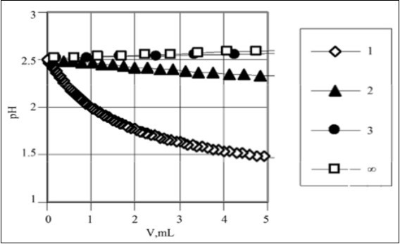
Generalizing, the D+T mixture may appear pH = const. during the titration T(V) ⇨ D(V0) only at defined relation between molar concentrations of components in D and T, as presented below.
Formulation of the Isohydricity Conditions – Examples
Example 1. HB (C) ⇨ HL (C0) and HL (C0) ⇨ HB (C)
The simplest isohydric system is composed of a strong monoprotic acid HB and a weak monoprotic acid HL with K1 expressed by Eq. 2. We derive first the isohydricity relation for the titration HB (C,V) ⇨ HL
(C0,V0), where V0 of C0 mol/L HL is titrated with V mL of C mol/L HB; V is the total volume of HB (C) added up to a defined point of the titration. From charge and concentration balances
[H+1] – [OH-1] = [B-1] + [L-1] ….(3)
[B-1] = CV/(V0+V) ….(4)
(HL) + (L-1) = C0V0/(V0+V) ….(5)
we get
[H+1] – [OH-1]  ….(6)
….(6)
where
 …….(7)
i.e.,
 …..(8)
(see Eq. 2).
Mixing the solutions according to titrimetric mode can be made in quasistatic manner, under isothermal conditions; it enables some changes in equilibrium constants, affected by thermal effects, to be avoided. As will be seen later, the ionic strength (I) of the related mixture is also secured; it acts in favour of constancy of K1 (Eq. 2) and KW = [H+1][OH-1] values. This way, the terms: [H+1] – [OH-1] = [H+1] – KW/[H+1] and  (Eq. 8) in Eq. 5 are constant at any V- value. In particular, at the start for the titration, V = 0, from Eq. 6 we have
[H+1] – [OH-1]= (1-n)⋅C0 (9)
(9)
Comparing the right sides of Equations 6 and 9, we get, by turns:

From Equations 9, 10
[H+1] – [OH-1]= C….(11)
From Equations 8, 10
K1/[H+1] + K1 = C/C0 ⇨ [H+1] = K1 ⋅ (C0/C-1) …..(12)
[OH-1] = KW/K1⋅ (C0/C-1)-1 ….(13)
Assuming [H+1] >> [OH-1] in Eq. 11, from [H+1] = C, and Eq. 12 we get
K1 ⋅ (C0/C-1)= C ⇨ C0 = C+C2/K1⇨ C0 = C+C2 ⋅ 10pk1 …...(14)
Alternately, after insertion of Equations 12 and 13 in Eq. 11 we have
K1⋅ (C0/C-1) - KW/K1⋅ (C0/C-1) = C
Denoting K1⋅(C0/C-1)= y, we have: y – KW/y – C = 0 ⇨ y2 – C⋅y – KW = 0 ⇨ y = C/2 ⋅ (1+(1+4KW/C2)1/2) ...(15)
as the positive root. At 4KW/C2<< 1, from Eq. 15 we get y = C, i.e.
K1⋅ (C0/C-1) = C …..(16)
and then we obtain Eq. 14 again.
After mixing isohydric solutions of HL and HB at any proportion, the degree of HL dissociation (see Eq. 8)

(see Eq. 1) is not changed.
The property, expressed by Eq. 14, was formulated first by Michałowski for different pairs of acid-base systems 3, 4, then generalized on more complex mixtures, and extended on mixtures containing basal salts and binary-solvent media 4, 17. Moreover, the isohydricity concept was the basis for a very sensitive method of determination of dissociation constants values 3, 4.
Identical formula is obtained for reverse titration, HL (C0,V) ⇨ HB (C,V0), where V0 of C mol/L HB is titrated with V mL of C0 mol/L HL. From Eq, 2 and [B-1] = CV0/(V0+V) , HL + [L-1] = C0V/(V0+V), we get, by turns,

at [H+1] >> [OH-1]. Then we have Eq. 10, and then Eq. 14. It means that the isohydricity condition is fulfilled for the set (C0, C, pK1), where Eq. 14 is valid, independently on the volume V of T added; it is identical for titrations: HB (C,V) ⇨ HL (C0,V0) and HL (C0,V) ⇨ HB (C,V0).
The related curves expressed by Eq. 14 are plotted in Figure 2, for different pK1 within (pC, pC0) coordinates. The curves appear nonlinearity for lower pK1 values and are linear, with slope 2, for pK1 greater than ca. 6. This regularity can be stated from Eq. 14 transformed as follows:
Figure 2.The plots of pC0 = – logC0 vs. pC = – logC relationships obtained on the basis of Eq. 14, for different pK1 values indicated at the corresponding lines 3.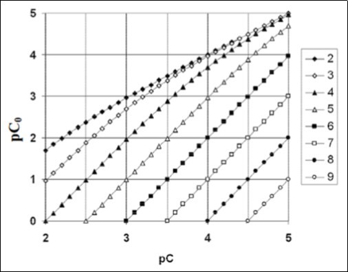
C0 = C2/K1 ⋅ (1+K1/C) ⇨
pC0 = 2 ⋅ pC - pK1 - log (1+10pC-pK1)….(17)
and valid for K1/C <<1 .
It can also be noticed that ionic strength (I) in the isohydric system (HB, HL) remains constant during the titration, i.e., it is independent on the volume V of the titrant T added. Namely, at [H+1] >> [OH-1], from Equations 3, 11 we get [7]
I = 0.5([H+1] + [B–1] + [L–1]) = C…..(18)
It is the unique property in titrimetric analyses, exploited in the new method of pK1 determination, suggested in 3, 4. According to Debye–Hückel theory, the constancy in ionic strength (I) is, apart from constancy in temperature T and dielectric permeability Ԑ, one of the properties securing constancy of K1 and KW values. The systems of isohydric solutions (HL, HB) have then a unique feature, not stated in other acid-base systems; it is the constancy of ionic strength (I), not caused by presence of a basal electrolyte 19, 20, 21, 22, 23, 24.
Other Pairs of Isohydric Solutions
The isohydricity concept can be extended on other T (V) ⇨ D (V0) systems, exemplified below.
Example 2. H2SO4 (C) ⇨ HCl (C0)
From the balances:
α - [HSO4-1] - 2[SO4-2] - [CI-1] = 0;
[HSO4-1] + [SO4-2] = cv/(V0+V); [CI-1] = C0V0/(V0+V)
we get the relation
 ….(19)
where  is the mean number of protons H+1 attached to SO4-2

At V = 0, from Eq. 19 we have C0 = [H+1] at H+1] >> [OH-1]. Then we obtain, by turns,

Example 3. NaHSO4 (C) ⇨ HCl (C0)
From the balances:

We get the relation

At V = 0, from Eq. 22 we have C0 = [H+1] at [H+1] >> [OH-1]. Then we obtain, by turns,
Example 4. Ba(OH)2 (C) ⇨ NaOH (C0)
From the balances:

We get the relation
 …..(24)
where

At V = 0, from Eq. 24 we have C0= [OH-1] at [H+1] <<[OH-1]. Then we obtain, by turns,

Example 5. Na2CO3 (C) ⇨ NaOH (C0)
From the balances:

we get the relation

where :

K1 = [H+1][HCO3-1]/[H2CO3], K2 = [H+1][CO3-2]/[HCO3-1]
At V = 0, from Eq. 26 we have C0 = - α = [OH-1] at [H+1] << [OH-1]. Then we get, by turns,
Example 6. CClH2COOH (C1) + CClH2COONa (C2) ⇨ HCl (C0)
From the relations:

we have, by turns:

At V = 0, from Eq. 28 we have C0 = α = [H+1] at [H+1] >> [OH-1]. Then we get, by turns,
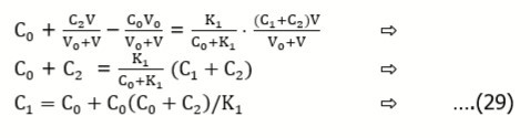

For example, at pK1 = 2.87, C1 = 0.1, C2 = 0.05, from Eq. 30 we get C0 = 0.002505. For pK1 = 2.87, C0 = 0.025, C2 = 0.05, from Eq. 29 we get C1 = 0.0998.
In further examples: 7 – 10 we apply the notation

where
[H+1][L(i)-1] = K1i[HL(i)] (i=1,2) ; [H+1][L(3)] = K13[L(3)H+1]
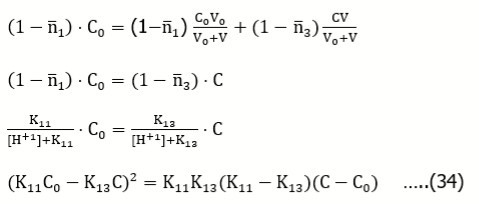
Example 7: HL(2) (C) ⇨ HL(1) (C0)
From the balances:

we get

For V = 0, at [H+1] >> [OH–1], from Eq. 31 we have [H+1] = and then, by turns,
Example 8: L(3)HB (C) ⇨ HL(1) (C0)
From the balances:

we get
For V = 0, at [H+1] >> [OH–1], from Eq. 33 we have [H+1] =  and then, by turns,
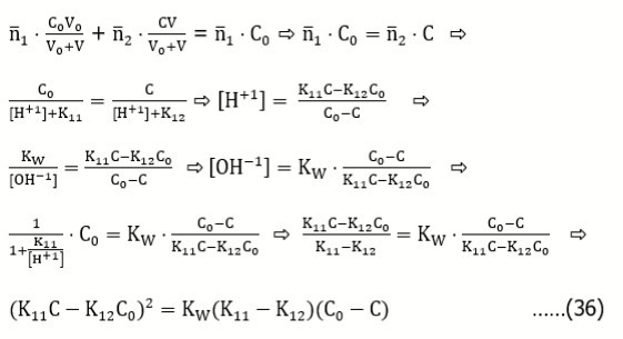
Example 9: ML(2) (C) ⇨ ML(1) (C0)
From the balances:

we get

For V = 0, at [OH–1] >> [H+1], from Eq. 35 we have [OH-1] =  and then, by turns,
Example 10: L(3) (C) ⇨ ML(1) (C0)
From the balances:

we get


For V = 0, at [OH–1] >> [H+1], from Eq. 37 we have [OH–1] = and then, by turns:

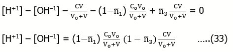
Example 11: (a) HB (C) ⇨ HnL (C0) and (b) HnL (C0) ⇨ HB (C)
Assuming that the acid HnL forms the species HiL+i-n (i = 0, 1, … , q), we get the charge and concentration balances:
 ….(39)

Applying the function
expressing the mean number of protons attached to the basic form L-n, where
from Eq. 39 we get , by turns :

Eq. 41 is also obtained for the reverse titration (b), where we get, by turns:

Assuming [H+1] >> [OH-1], from Eq. 42 we get [H+1] = C. Putting it into (3), from (7) we get
 …..(43)
In particular, for q = n = 1, K1 = 1/K1H, from Eq. 43 we get the relation

transformed into Eq. 14.
Isohydricity in Terms of Conductometric and pH Titrations
The diversity in meaning the isohydricity term, referred to pH and conductivities, made an inevitable inconsistency/controversy, indicated above. Conductivity κ = 1/ρ (ρ – resistivity) of a solution is a sum of terms involved with all cationic and anionic species contributing the current passing through the solution 25
 …...(44)
where zi – charge (in elementary charge units), and ui – ionic mobility for i-th ionic species, Xjzi, F – Faraday constant; each ion contributes a term proportional to its concentration [Xjzi]. The property (44) is valid at low concentrations, where interactions between ions can be neglected. Ionic interactions in more concentrated solutions can alter the linear relationship between conductivity and concentrations. Denoting |zi|·ui·F = ai, for ionic species composing the HB + HL mixture considered in Example 1, we have the formula 4
k = a1⋅[H+1] + a2⋅[B-1] + a3⋅[L-1]…..(45)
From the simplified charge balance [H+1] = [L-1] + [B-1], valid at [H+1] >> [OH-1], from Eq. 45 it results that
k = (a1+a2)⋅[B-1] + (a1+a3)⋅[L-1]…..(46)
Assuming, for a moment, thata2 = a3, from Eq. 46 we have
K = (a1+a3)⋅[B-1] + [L-1]) = (a1+a3)⋅[H+1] = (a1+a3)⋅10-pH = const…..(47)
at pH = const. At constant ionic strength I (this property is immanent in such isohydric system, see Eq. 18), a1 and a3 are not changed during the titration/mixing. However, the assumption a2 = a3 is not valid, in general 4.
In experimental part of the paper, the results from pH titrations (in aqueous and mixed-solvent media) will be compared with results from conductometric titrations.
The Isohydric Method of Acidity Constant Determination
The conjunction of properties: pH = const, I = const, together with constancy of temperature (T = const), as stated above, provided a useful tool for a sensitive method of determination of pK1 values for weak acids HL, as indicated and applied in 3, 4. This method is illustrated with some examples taken from 4.
The isohydricity property can be perceived as a valuable tool applicable for determination/validation 3, 4 of pK1 for a weak acid HL. For this purpose, a series of pairs of solutions {HB (C), HL (C0i*)} (i=1,…,n) is prepared, where C and C0i* are interrelated in the formula
 …..(48)
where pk1i* (i = 1,…, n) are the numbers chosen from the vicinity of the true (expected, correct) pK1 value for HL (compare with Eq. 14). From Equations 14 and 48 we have the relation
 …….(49)
The principle of the method is illustrated in Figure 3, where simulated titration curves pH = pH(V) are obtained for titrations HB (C) ⇨ HL (C0i*) related to different C0i* values at constant C value. As we see, a misfit DpKi = pK1i* – pK1 between real (pK1) and pre-assumed (pK1i*) values for acidity constant causes a non-parallel, to V-axis, course of the related curve pH = pH(V); the curve/line is parallel to the V-axis only for pK1* = pK1, at C0* = C0 = C + C2·10pk1.
Figure 3.The pH vs. V relationships plotted for the titration HB (C) ⇨ HL (C0i*) at pK1 = 2.87 for HL; V0 = 3, C = 0.01, C0i* calculated from Eq. 48 at indicated pK1i* values.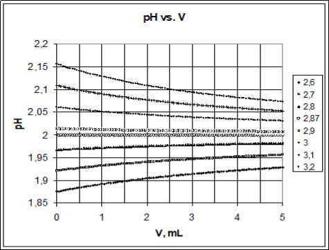
Experimental Data
pH-Metric Titrations
The validity of some models presented above were verified and confirmed by results of pH-metric and conductometric titrations T (V) ⇨ D (V0), presented in 4. In the present article, we refer to the results of titrations of (1) chloroacetic acid (HL = CH2ClCOOH) and (2) mandelic acid (HL = C6H5CH(OH)COOH) solutions as titrands with HB = HCl (C) as the titrant. All technical details of these titrations are specified therein 4. The pH titrations considered here are as follows.
(1) pH titration HCl (C) ⇨ CH2ClCOOH (C0i*)
(2) pH titration HCl (C) ⇨ C6H5CH(OH)COOH (C0i*)
The C and C0i* (i=1,…,5) values are collected in Table 1 and Table 1. For example, at C = 0,00965 and pK11* = 2,65, we have C01* = 0,051246; at C = 0.00472, pK11* = 3.10 we get C01* = 0.032767. The C0i* values were calculated from Eq. 48 for pK1* values taken from the vicinity of the related pK1 value known from the literature data.
Table 1. The data related to pH-titrations with chloroacetic acid (C0i*) in D.| HL = chloroacetic acid | ||||
| pK1i* | C | C0i* | a | b |
| 2,65 | 0.00965 | 0.05125 | 2.04646 | -0.00942 |
| 2,75 | 0.00965 | 0.06202 | 2.02252 | -0.00692 |
| 2.87 | 0.00965 | 0.07868 | 1.95490 | -0.00162 |
| 2.97 | 0.00965 | 0.09643 | 1.90275 | 0.00664 |
| 3.10 | 0.00965 | 0.1269 | 1.83071 | 0.01105 |
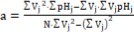
The pH titrations HB (C) ⇨ HL (C0i*) were made at V0 = 3 mL of D and T added up to V = 4 mL. The exact pK1o value was searched here according to interpolation procedure. The results of titrations (Figure 4a, b) are approximated by straight lines pH = a + b·V (see Figure 5a, b), where b=bi is the slope of the related line (i=1,…,5). The coefficients a and b are calculated according to least squares method from the formulae:
Figure 4.The pH vs. V relationships for (5a) HL = chloroacetic acid and (5b) HL = mandelic acid, plotted for indicated pK1* = pK1i* (i = 1,…,6) values. For further details see Tables 1 and 2 4.
Figure 5.The b vs. pK1* relationships (Eq. 52) found for (5a) chloroacetic and (5b) mandelic acids, see Tables 1, 2.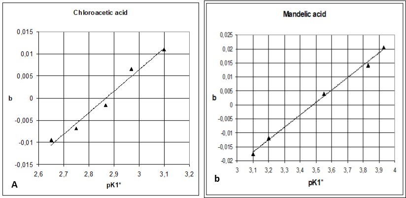
 …...(50)
 …….(51)
where

For example, linear approximation of the curve in Figure 4b obtained at pK11* = 3.10 (see Table 2) gives the line pH = 2.48438 – 0.01766·V, The value s = 0.0036 obtained for this approximation from the formula s=(s2)1/2,where 
| HL = mandelic acid | ||||
| pK1i* | C | C0i* | a | b |
| 3.10 | 0.00472 | 0.03277 | 2.48438 | - 0.01766 |
| 3.20 | 0.00472 | 0.04003 | 2.43421 | - 0.01197 |
| 3.55 | 0.00472 | 0.08377 | 2.28123 | 0.00393 |
| 3.83 | 0.00472 | 0.15534 | 2.12521 | 0.01417 |
| 3.93 | 0.00472 | 0.19434 | 2.06462 | 0.02054 |
(where N=200 – number of experimental points (Vj, pHj)) from the V-interval < 0, 4 > is comparable with precision of pH-measurements. Note that the curve at pK11* = 3.10 (Figure 4b) has relatively great curvature.
The slopes b, obtained from the series of n = 5 titrations were applied for evaluation of the true pK1 = pK1o value. Assuming the linear relation between b = bi and pK1* = pK1i*, we apply the regression equation
 …..(52)
where i = 1,…,n; n = 5. Then we have:
Where  For example, α = – 0.13954, β = 0.048647 in the relation specified at the bottom of Table 1; then we have pK1* = pK1o = 0.13954/0.048647 = 2.868 at b = 0.
The pK1o values are related to b = 0. In both cases, an additional, 6th titration made for pK16* = pK1o, obtained by interpolation, confirmed the adequacy of this evaluation (see Figure 4a, 4b).
The experimental value for pK1o = 2.868 referred to chloroacetic acid agrees with the one cited in literature: 2.87 26, 27, 2.82 28, 2.85 29, 30, 2.86 31. For mandelic acid, pK1o = 3.481 lies within the wide interval: from 3.4132 to 3.85 29, 33.
Comparison of Results Obtained from Conductometric and pH Titrations
The results of pH titrations presented in Figure 4a and 4b can be compared with results of conductometric titrations specified in 4 for the (HCl, HL) systems with (a) HL = chloroacetic acid (CA), (b) HL = mandelic acid (MA). First, one can state that the conductomeric titration curves are arranged in the reverse order than pH titration curves, from the viewpoint of changes in C0i* values; this is understandable because higher pH values correspond to lower [H+1] values. Moreover, the conductometric titration curves have more regular course than pH titration curves. At pK1i* = 2.87, the pH titration curve for CA is nearly parallel to V-axis (Figure 4a), whereas for conductometric titration the parallel course can be ascribed to the line obtained at pK1i* ca. 2.90. For MA, the parallel course of conductometric titration occurs at pK1i* = 3.55 (Figure 4b), whereas from results of pH titrations the value pK1* = 3.481 was obtained (Table 1); the pH titration curve for MA at pK1i =3.55 is not parallel to V-axis (Figure 4a). This means that a2 for Cl-1 (see Eq. 47) differs from a3 for anions L-1 related to CA and MA, respectively. However, the differences are not too large and the conductometric titration, offering more regular course of the respective curves, can be considered as a reasonable alternative to the pH titration made within the isohydric method of pK1 determination.
Different Aspects and Meanings of Isohydricity
Constancy of pH during addition of one of the solutions forming the isohydric system into another one recalls the concepts of buffering action and the dynamic buffer capacity βV = |dc/dpH| 1, 2, 34, 35, 36. Isohydric systems are characterized by extremely high βV value. Referring e.g. to addition of V mL of titrant T mol/L HL (C) into V0 mL of C0 mol/L HB, we apply c = CV/(V0+V); in ideal case βV . The isohydricity is not directly relevant to buffering action; nevertheless, it is on–line with a general property desired from buffering systems. The isohydricity concept is also in some relevance with pH-static titration 37, 38 principle. Moreover, the isohydricity concept is referred to acid-base homeostasis in living organisms 39, 40. In biology, it is used for describing plants that limit transpiration in order to maintain a constant amount of water in the leaves 41, 42, 43, 44. The isohydric principle has special relevance to in vivo biochemistry, where multiple acid-base pairs are in solution.
Some acids involved in redox (e.g. HClO, HBrO) and complexation equilibria do not meet the conditions imposed by the isohydricity property, see e.g. 45, 46, 47, 48, and other authors’ references cited therein.
Final Comments
The formulation referred to the isohydric D+T acid-base systems formed from D and T of different complexity was presented. Particularly, the titration in (HL, HB) system may occur at constant ionic strength (I) value, not resulting from presence of a basal electrolyte. This very advantageous conjunction of the properties provides, among others, a new, very sensitive method for verification of pK1 value for HL. The method was tested experimentally on (HL, HCl) systems in aqueous and mixed-solvent media, and compared with the literature data. Some useful (linear and hyperbolic) correlations were applied for pK1 validation purposes.
The isohydric method, formulated on the basis of isohydricity property, is also a proposal for use in physicochemical laboratories, as a sensitive tool for the determination of dissociation constants of weak acids HL, especially ones with small pK1 values, for which the standard method of pK1 determination based on inflection point location on the related titration curve obtained for (HL, MOH) system is not applicable 4. The reference of isohydricity to conductometric titrations was also discussed in context to the pH-metric titration.
References
- 1.Asuero A G, Michałowski T. (2011) Comprehensive formulation of titration curves referred to complex acid-base systems and its analytical implications. Critical Reviews in Analytical Chemistry .http://www.tandfonline.com/toc/batc20/41/2 41(2), 151-187.
- 2.Michałowski T.Asuero AG (2012) New approaches in modelling the carbonate alkalinity and total alkalinity. Critical Reviews in Analytical Chemistry,.http://www.tandfonline.com/toc/batc20/42/3 42(3), 220-244.
- 3.Michałowski T, Pilarski B, Asuero A G, Dobkowska A. (2010) A new sensitive method of dissociation constants determination based on the isohydric solutions.
- 4.Asuero A G, Pilarski B, Dobkowska A, Michałowski T. (2013) On the isohydricity concept – some comments. , Talanta.http://www.ncbi.nlm.nih.gov/pubmed/23708536.112: 49-54.
- 5.Arrhenius S. (1888) . Theorie der isohydrischen Losungen, Zeitschrift für Physikalische Chemie.2: 284.
- 6.Bancroft W D. (1900) Isohydric Solutions. , Journal of Physical Chemistry.https://pubs.acs.org/doi/pdf/10.1021/j150022a003 4(4), 274-289.
- 7.Michałowski T.Asuero AG. (2012).Formulation of the system of isohydric solutions,JournalofAnalyticalSciences,MethodsandInstrumentation.
- 9.Arrhenius S. (1887) Wiedemann's Annalen 30: 51; a cit. in Arrhenius S (1889), Theory of isohydric solutions, Philosophical Magazine Series.
- 10.Arrhenius S.(1889) Theory of isohydric solutions, The London, Edinburgh. , and Dublin Philosophical Magazine and Journal of Science, Series.5
- 12.Sørensen S. (1909) Enzymstudien II: Uber die Messung und die Bedeutung der Wasserstoffionenkonzentration bei enzymatischen Prozessen. , Biochemische Zeitschrift 21, 131-200.
- 14.Carpéni G. (1968) Recherches sur le point isohydrique et les équilibres acido-basiques de condensation ou association en chimie. XXVI. Quelques nouvelles remarques et commentaires théoriques. , Canadian Journal of Chemistry
- 16.R De Levie. (2005) On isohydric solutions and buffer pH. , Journal of Electroanalytical Chemistry
- 17.A M Michałowska-Kaczmarczyk, Spórna-Kucab A, Michałowski T. (2017) Principles of Titrimetric Analyses According to Generalized Approach to Electrolytic Systems (GATES), in:. Advances in Titration Techniques, Vu Dang Hoang (Ed.) InTech Chap .
- 18.Pilarski B, Dobkowska A, Foks H, Michałowski T. (2010) Modelling of acid–base equilibria in binary-solvent systems:.
- 19.Michałowski T, Rokosz A, Tomsia A. (1987) Determination of basic impurities in mixture of hydrolysable salts. , Analyst
- 20.Michałowski T. (1988) Possibilities of application of some new algorithms for standardization purposes; Standardisation of sodium hydroxide solution against commercial potassium hydrogen phthalate.
- 21.Michałowski T, Rokosz A, Negrusz-Szczęsna E. (1988) Use of Padé approximants in the processing of pH titration data; Determination of the parameters involved in the titration of acetic acid. , Analyst 113, 969-972.
- 22.Michałowski T, Rokosz A, Kościelniak P, Łagan J M, Mrozek J. (1989) Calculation of concentrations of hydrochloric and citric acids together in mixture with hydrolysable salts. , Analyst 114, 1689-1692.
- 23.Michałowski T. (1992) Some new algorithms applicable to potentiometric titration in acid-base systems. , Talanta 39, 1127-1137.
- 24.Michałowski T, Gibas E. (1994) Applicability of new algorithms for determination of acids, bases, salts and their mixtures. , Talanta 41, 1311-1317.
- 30.Dawa B A, Gowlan J A. (1978) Infrared studies of carboxylic acids and pyridine in chloroform and methanol. , Can. J. Chem.https://www.nrcresearchpress.com/doi/pdfplus/10.1139/v78-421 56, 2567-2571.
- 32.Klingenberg J J, Knecht D S, Harrington A E, Meyer R L. (1978) Ionization constant of mandelic acid and some of its derivatives. , Journal of Chemical and Engineering Datahttps://pubs.acs.org/doi/pdf/10.1021/je60079a024 23, 327-328.
- 34.Michałowska-Kaczmarczyk A M, Michałowski T. (2015) Buffer Capacity in Acid-Base Systems,JournalofSolutionChemistry.
- 35.Michałowska-Kaczmarczyk A M, Michałowski T, Asuero A G. (2015) Formulation of dynamic buffer capacity for phytic acid,AmericanJournalof hemistryandApplications.
- 36.Michałowska-Kaczmarczyk A M, Spórna-Kucab A, Michałowski T. (2017) Dynamic Buffer Capacities in Redox Systems,JournalofChemistryandAppliedChemicalEngineering.
- 37.Michałowski T, Toporek M, Rymanowski M. (2007) pH-Static Titration: A Quasistatic Approach. , Journal of Chemical Education.http://pubs.acs.org/doi/abs/10.1021/ed084p142 84, 142-150.
- 38.Michałowski T, Asuero A G, Ponikvar-Svet M, Toporek M, Pietrzyk A et al. (2012) Principles of computer programming applied to simulated pH–static titration of cyanide according to a modified Liebig-Denigès method. , Journal of Solution Chemistry.http://link.springer.com/article/10.1007%2Fs10953-012-9864-x 41(7), 1224-1239.
- 39.Banerjee A. Clinical Physiology:An Examination Primer,Cambridge University Press,Cambridge (2005) .
- 40.Hamm L L, Nakhoul N, Hering-Smith K S. (2015) Acid-Base Homeostasis,ClinicalJournaloftheAmericanSocietyofNephrology.
- 41.Attia Z, Oren R DomecJ-Ch.Way DA,MoshelionM.(2015).Growth and physiological responses ofisohydricandanisohydricpoplars to drought,Journal of Experimental Botany.
- 42.Dan-Dan L, Chuan-Kuan W, Ying J. (2017) Plant water-regulation strategies: Isohydric versus anisohydric behavior,ChineseJournalofPlantEcology.http://www.plant-ecology.com/EN/10.17521/cjpe.2016.0366.41(9):. 1020-1032.
- 43.Garcia-Forner N, Biel C, Savé R, Martínez-Vilalta J. (2017) Isohydric species are not necessarily more carbon limited than anisohydric species during drought,Tree Physiology.
- 44.Coupel-Ledru A, Tyerman S D, Masclef D, Lebon E, Christophe A et al. (2017) Abscisic Acid Down-Regulates Hydraulic Conductance of Grapevine Leaves in Isohydric Genotypes Plant Physiology.
- 45.Michałowska-Kaczmarczyk A M, Michałowski T.(2019).The new paradigm in thermodynamic formulation of electrolytic systems – A review. , Archive of Biomedical Science and Engineering.https://www.peertechz.com/articles/ABSE-5-113.pdf.5(1): 19, 61.
- 46.Michałowska-Kaczmarczyk A M, Michałowski T. (2018) distinguishing role of 2.f(O) - f(H). in electrolytic