
The Fermi-Pasta-Ulam Quantum Recurrence in The Dynamics of an Elementary Physical Vacuum Cell and The Problem of its Polarization
Abstract
A model of a Quantum recurrence in the dynamics of an elementary physical vacuum cell within the framework of four coupled Shrodinger equations has been suggested. The model of an elementary vacuum cell shows that a Quantum recurrence which represents the dynamics of virtual transformations in the cell, qualitatively differs from that of Poincare and the Fermi-Pasta-Ulam. Whereas these recurrences develop in time or space, the Quantum recurrence develops in a sequence of Fourier images represented by non exponentially separating functions. The sequence experiences random energy additions but no exponential separation occurs. The Quantum recurrence can be defined as the most frequent array of Fourier images that appear in a certain quantum system during a period of its observation. Different scenarios of the Fourier images sequences interpreted as bosons (electron and positron) and fermions (photons) apearing in the solutions of the model demonstrate that during some periods of its observation they become indistinguishable. The quantum dynamics of every physical vacuum cell depends on the dynamics of many other vacuum cells interacting with it, thus the quasi periodicity (during the period of observation) of the Fourier images recurrence can have infinite periods of time and space and the amplitudes of the Fourier images can vary many orders in their magnitudes. Such recurrence times does not correspond even roughly to the Poincare recurrence time of an isolated macroscopic system. It reminds the behavior of spatially coupled standard mappings with different parameters. The amount of energy in the physical vacuum is infinite but extracting a part of it and converting, it into a time-space form requires a process of periodical transfer of the reversible microscopic system dynamics into that of a macroscopic system. This process can be realized through a resonant interaction between the classical and quantum recurrences developing in these two systems. However, a technical realization of this problem is problematic.
Article Information
- Received
- Accepted
- Published
Academic Editor: Loai Aljerf, Department of Basic Sciences, Faculty of Dental Medicine, Damascus University, Damascus, Syria.
Checked for plagiarism: Yes
Review by: Single-blind
Copyright © 2020 Berezin. A. A
 This is an open-access article distributed under the terms of the Creative Commons Attribution License, which permits unrestricted use, distribution, and reproduction in any medium, provided the original author and source are credited.
Corresponding author: Berezin A. A., Independent researcher, Moscow, Russia —
Competing Interests
The authors have declared that no competing interests exist.
Funding
No specific funding statement was provided by the authors.
Data Availability
No data-availability statement was provided by the authors.
Citation:
Introduction
After Poincare had stated his classical form of a recurrence when both an amplitude and a phase of the system must recur after a certain period of time to their initial states 1 Fermi, Pasta and Ulam discovered in a system of non linearly coupled oscillators 2 a much more sophisticated form of recurrence when the recurrences to the initial states were not identical but manifested the appearance of stochasticity in the process of energy regrouping in a sequence of different recurrences. Its further studies 3, 4 have induced a following theoretical and experimental research aimed at a search for specific recurrence properties in quantum systems.
In a quantum case, the notion of a phase space trajectory loses its meaning and so does the notion of the Lyapunov exponent, which measures the separations between trajectories 5. When a discrete energy spectrum is present, the exponential separation is excluded even for expectation values of observables, on time scale on which level spacings are resolvable. The dynamics here is characterized by quasiperiodicity, i.e. recurrences rather than chaos in the classical sense. In contrast to classical chaos, quantum mechanical regular motion cannot be characterized by high sensitivity to small changes of initial conditions, Due to unitarity of quantum dynamics, the overlap of two wave functions remains time independent, provided the time dependence of both wave functions is generated by the same Hamiltonian. For periodically driven systems, the Hamiltonian has a variable parameter. All these are generically nonintegrable classically. However, in case of a kicked rotator 5 even under conditions of fully developed classical chaos it does not display the energy level repulsion. The kinetic energy and hence the quantum mechanical momentum uncertainty does not follow the classical diffusive growth indefinitely. After a certain break time the quantum mean enters a mode of quasiperiodic behavior. It brings to the idea that classical and quantum recurrence behaviors should look different.
Model
We consider a possible existence of a quantum recurrence in a model of the following virtual reaction taking place in the physical vacuum:
 (1)
(1)
Equation (1) describes a reversible electromagnetic formation of an electron-positron couple from two photons together with electron-positron annihilation giving a birth to two photons.
We discuss the usage of Anderson's model of a particle whose possible locations are the equidistant sites of a one-dimensional chain 6. In our case, these are electron or positron in (1). At each site a random potential Vm from neighboring reactions acts and the hopping of the particle from one site to its r-th neighbor is described by a hopping amplitude Wr. The probability amplitude pm for finding the particle on the m-th site obeys the Shrodinger equation 6:
 (2)
(2)
Consider if Vm are random numbers uncorrelated from site to site and distributed with a density ρ(Vm). The hopping amplitudes Wr, in contrast, will be taken to be nonrandom and to decrease fast for hops of increasing length r. As it was shown 5, 7 this case can be reduced to the standard mapping form. On the other hand, the process of interaction between a photon and electron or positron can be interpreted as a random one, which represents either penetrating of a photon through or reflecting from a potential barrier of the electron or positron field. That brings to the temporal form of coupled Shrodinger equations:

(3)
Where ψph+is the amplitude that photon will tunnel the barrier and ψph- is the amplitude that a photon will be reflected from the barrier. K –characterizes the potential barrier.
The system (3) was used for a description of the Josephson junction dynamics 8.The process described by (3) also can be interpreted as a kicked rotator and can be reduced to the standard mapping form. Together with this some popular examples of chaos are of this type 9
Summing up one can see that the two quantum problems (2) and (3) can be reduced to the standard mapping form. In the paper 10 there was suggested a model of the Fermi-Pasta-Ulam recurrence within the framework of two coupled high and low frequency standard mappings. This approach looks perspective for describing recurrences in quantum systems just like (1). Since the vacuum cell (1) is under the influence of similar cells the processes of the energy addition to and subtraction from the cell have to be included into the model. For this purpose, the Pippard's idea about the Shrodinger equation with a complex potential has been used 11. He suggested the description of a particle moving in a potential field: -iVn through the following form of the Shrodinger equation:
 (4)
(4)
If ψ = 0 when x=0 and x=a, for an eigenvalue with a number n for which ψn = sin(nπ/a), a following equality must be fulfilled:

Therefore a full wave function: 
possesses a dissipation proportional to: 
An impulse response of this system, which corresponds to an addition of the other eigenvalue states after the impulse, in a general case (due to such members as ψm*ψn) has the members varying as  and describing the oscillations at the frequency of beatings and decaying as
  If to take the dimensions of electron and positron in a coupled state (1) as symmetrical ones (-a+a), their wave functions can be described within the framework of coupled spatial Shrodinger equations having different directions of a spatial variable and having random potentials reflecting the influence of other cells like (1). Two coupled photons in (1) are described within the framework of coupled temporal Shrodinger equations (3) having different directions of a time variable and also having random potentials. The link between the two couples is realized through a mutual parametric excitation by the differences between the wave functions of electron and positron and that of between the two photons. The differences have opposite signs in the coupled couples of the Shrodinger equations because of mentioned opposite directions of a spatial and temporal coordinates there. Since the number of the virtual reactions similar to (1) is infinite and they are interconnected through random potentials, we have to insert them into the coupled Shrodinger equations. Generally, the energy damping-increasing process is interpreted as a resonant chaotically reversible exchange of energy between the vacuum cells like (1).
Accounting all mentioned the reaction (1) can be described by four coupled Shrodinger equations:

(5)
Where ψ1 - is the wave function of electron in (1), ψ2 - is the wave function of the first photon in (1), ψ3 - is the wave function of the second photon in (1), ψ4 - is the wave function of a positron in (1). E1,E2,E3,E4 are random magnitudes of energy which correspond to the chaotically reversible exchange of energy between the vacuum cells. The multiplied wave function members in (1) reflect the non linear interaction processes. Vrandom1,Vrandom2,Vrandom3,Vrandom4 are random potentials.
For numerical analysis the system (3) was reduced to four coupled differential equations of the second order:

(6)
Where e(t),p(t) correspond to the electron and positron wave functions ψ1, ψ4 in (5), and h(t),r(t) correspond to the wave functions of two photons ψ2, ψ3 in (5);
R1, R4 are random functions distributed within the interval (-1,1) corresponding to the positive and negative dispersion processes in the first and fourth equations in (5) having place due to energy interactions of electrons and positrons with other cells like (1); R2, R3 are random functions distributed within the interval (-1,1) corresponding to the dissipation processes in the second and third equations in (5) having place due to resonant interactions of photons with other cells like (1) 11; A1,A2,A3,A4 are random functions distributed within the interval (0,1) corresponding to the random potentials Vrandom1,Vrandom2,Vrandom3,Vrandom4 in (5); C1, C2, C3, C4 are positive constants. Spatial and temporal symmetries in (5) are realized in (6) through a symmetrical resulting Fourier transform image of the functions e, p, h, r in relation to the frequency axis (consequence of aliasing); ω1 corresponds to the spatial frequency in Eq. 1,4 in (5); ω2 corresponds to the temporal frequency in Eq. 2,3 in (5). To get the ratio between ω2 and ω1 we can equalize the energy for both spatial and temporal Shrodinger equations in (5).
Accounting that the electron and positron radius re,p= 2.8*10-13cm, temporal frequency/energy = 2.42*1014 Hz/e.v., spatial frequency/energy= 8.06*103cm-1/e.v.,and considering the length of spatial waves 4*re,pif an electron and positron are next to each other we can get the ratio between the temporal frequency ω2 in (5) and the spatial frequency ω1 in (5):

Accounting a quantum character of the dynamics in the cell (1) the initial conditions for the functions e, p, h, r were taken random.
Numerical Study of the Model
A factual opposite direction of spatial (Eq.1,4) and temporal (Eq.2,3) coordinates in the system (5) brings the numerical analysis of the system (6) to the statistical observing of the Fourier image similarities appearing quasi periodically in multiple runs of the computer program during the solving process of the system (6). Since the potentials, dissipative members and initial conditions in (6) were random every run gave different Fourier images. A few hundred runs coverage allowed revealing the most frequent sequences of the Fourier images appearing quasi periodically in the results of computer analysis of the system (6) and to give them interpretations. (Figure 1, Figure 2, Figure 3, Figure 4, Figure 5, Figure 6, Figure 7, Figure 8, Figure 9, Figure 10, Figure 11, Figure 12, Figure 13, Figure 14, Figure 15, Figure 16, Figure 17, Figure 18, Figure 19, Figure 20, Figure 21, Figure 22, Figure 23, Figure 24)
Figure 1. Symmetrical (relatively the centre of horizontal axis) Fourier images of the functions e and p interpreted as a beginning of the annihilation process. Vertical axis: amplitude, horizontal axis: number of steps. Units conditional.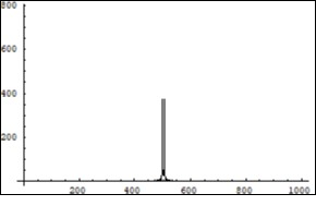
Download figure
Figure 2. Symmetrical (relatively the centre of horizontal axis) Fourier images of the functions h and r interpreted as a beginning of the two photons forming process. Vertical axis: amplitude, horizontal axis: number of steps. Units conditional.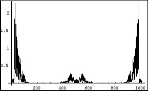
Download figure
Figure 3. Symmetrical (relatively the centre of horizontal axis) Fourier images of the functions h and r interpreted as a beginning of the two photons forming process. Vertical axis: amplitude, horizontal axis: number of steps. Units conditional.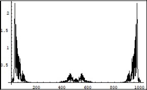
Download figure
Figure 4. Symmetrical (relatively the centre of horizontal axis) Fourier images of the functions e and p interpreted as a beginning of the annihilation process. Vertical axis: amplitude, horizontal axis: number of steps. Units conditional.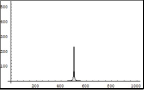
Download figure
Figure 5. Symmetrical (relatively the centre of horizontal axis) Fourier images of the functions e and p interpreted as a continuation of the electron and positron annihilation process. Vertical axis: amplitude, horizontal axis: number of steps. Units conditional.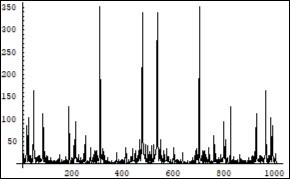
Download figure
Figure 6. Symmetrical (relatively the centre of horizontal axis) Fourier images of the function h interpreted as a multiphoton forming process. Vertical axis: amplitude, horizontal axis: number of steps. Units conditional.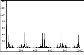
Download figure
Figure 7. Symmetrical (relatively the centre of horizontal axis) Fourier images of the function r interpreted as a completion of the two photons forming process. Vertical axis: amplitude, horizontal axis: number of steps. Units conditional.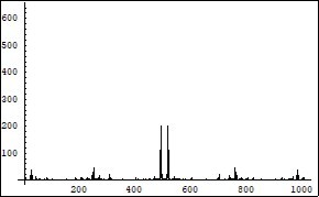
Download figure
Figure 8. Symmetrical (relatively the centre of horizontal axis) Fourier images of the functions e and p interpreted as a continuation of the electron and positron annihilation process. Vertical axis: amplitude, horizontal axis: number of steps. Units conditional.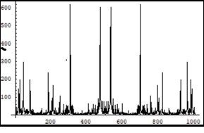
Download figure
Figure 9. Symmetrical (relatively the centre of horizontal axis) Fourier images of the functions e and p interpreted as a beginning of the two photon interaction process. Vertical axis: amplitude, horizontal axis: number of steps. Units conditional.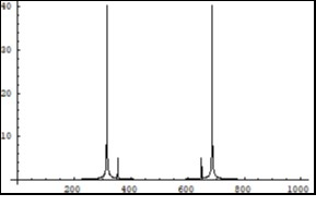
Download figure
Figure 10. Symmetrical (relatively the centre of horizontal axis) Fourier images of the functions h and r interpreted as a beginning of the two photon interaction process. Vertical axis: amplitude, horizontal axis: number of steps. Units conditional.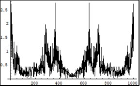
Download figure
Figure 11. Symmetrical (relatively the centre of horizontal axis) Fourier images of the functions h and r interpreted as a beginning of the two photon interaction process. Vertical axis: amplitude, horizontal axis: number of steps. Units conditional.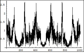
Download figure
Figure 12. Symmetrical (relatively the centre of horizontal axis) Fourier images of the functions e and p interpreted as a beginning of the two photon interaction process. Vertical axis: amplitude, horizontal axis: number of steps. Units conditional.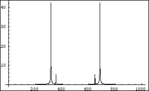
Download figure
Figure 13. Symmetrical (relatively the centre of horizontal axis) Fourier images of the functions e and p interpreted as an interaction process between electron, positron and photons. Vertical axis: amplitude, horizontal axis: number of steps. Units conditional.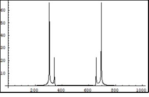
Download figure
Figure 14. Symmetrical (relatively the centre of horizontal axis) Fourier images of the functions h and r interpreted as an interaction process between photons and electron, positron. Vertical axis: amplitude, horizontal axis: number of steps. Units conditional.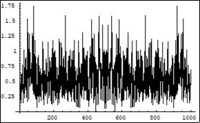
Download figure
Figure 15. Symmetrical (relatively the centre of horizontal axis) Fourier images of the functions h and r interpreted as an interaction process between photons and electron, positron. Vertical axis: amplitude, horizontal axis: number of steps. Units conditional.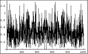
Download figure
Figure 16. Symmetrical (relatively the centre of horizontal axis) Fourier images of the functions e and p interpreted as an interaction process between electron, positron and photons. Vertical axis: amplitude, horizontal axis: number of steps. Units conditional.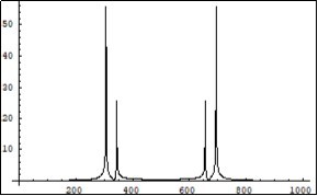
Download figure
Figure 17. Symmetrical (relatively the centre of horizontal axis) Fourier images of the functions e and p interpreted as a beginning of the electron-positron couple forming process. Vertical axis: amplitude, horizontal axis: number of steps. Units conditional.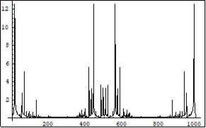
Download figure
Figure 18. Symmetrical (relatively the centre of horizontal axis) Fourier images of the functions h and r interpreted as a beginning of the two photon coupling process which results in a forming of the electron-positron couple. Vertical axis: amplitude, horizontal axis: number of steps. Units conditional.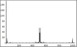
Download figure
Figure 19. Symmetrical (relatively the centre of horizontal axis) Fourier images of the functions h and r interpreted as a beginning of the two photon coupling process which results in a forming of the electron-positron couple. Vertical axis: amplitude, horizontal axis: number of steps. Units conditional.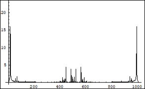
Download figure
Figure 20. Symmetrical (relatively the centre of horizontal axis) Fourier images of the functions e and p interpreted as a beginning of the electron-positron couple forming process. Vertical axis: amplitude, horizontal axis: number of steps. Units conditional.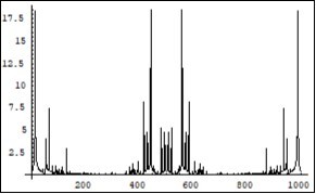
Download figure
Figure 21. Symmetrical (relatively the centre of horizontal axis) Fourier images of the function e interpreted as a beginning of the electron-positron wave functions overlapping process. Vertical axis: amplitude, horizontal axis: number of steps. Units conditional.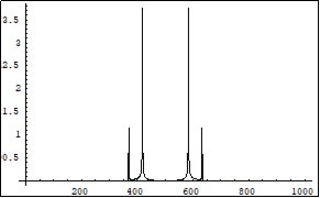
Download figure
Figure 22. Symmetrical (relatively the centre of horizontal axis) Fourier images of the functions h and r interpreted as an energy levels forming process as a result of the photons confinement in the overlapped electron-positron wave functions. Vertical axis: amplitude, horizontal axis: number of steps. Units conditional.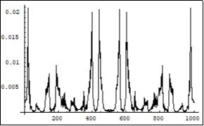
Download figure
Figure 23. Symmetrical (relatively the centre of horizontal axis) Fourier images of the functions h and r interpreted as an energy levels forming process as a result of the photons confinement in the overlapped electron-positron wave functions. Vertical axis: amplitude, horizontal axis: number of steps. Units conditional.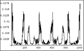
Download figure
Figure 24. Symmetrical (relatively the centre of horizontal axis) Fourier images of the function p interpreted as a middle of the electron-positron wave functions overlapping process. Vertical axis: amplitude, horizontal axis: number of steps. Units conditional.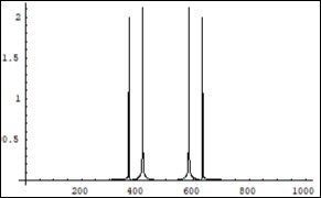
Download figure
One more numerical experiment was aimed at a possible application of the mathematical model. For that purpose all random functions R1, R2, R3, R4 in (6) were substituted by positive constants. The result of this artificial situation is given in. Figure 25, Figure 26, Figure 27, Figure 28.
Figure 25. Symmetrical (relatively the centre of horizontal axis) Fourier images of the functions e and p interpreted as a beginning of the annihilation process. The numerical study was carried out under constant (not random) positive dissipative coefficients R1, R2, R3, R4 in (6).Vertical axis :amplitude, horizontal axis: number of steps. Units conditional.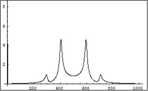
Download figure
Figure 26. Symmetrical (relatively the centre of horizontal axis) Fourier images of the functions h and r interpreted as a middle of the two photons forming process. The numerical study was carried out under constant (not random) positive dissipative coefficients R1, R2, R3, R4 in (6). Vertical axis: amplitude, horizontal axis: number of steps. Units conditional.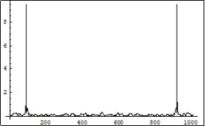
Download figure
Figure 27. Symmetrical (relatively the centre of horizontal axis) Fourier images of the functions h and r interpreted as a middle of the two photons forming process. The numerical study was carried out under constant (not random) positive dissipative coefficients R1, R2, R3, R4 in (6). Vertical axis: amplitude, horizontal axis: number of steps. Units conditional.
Download figure
Figure 28. Symmetrical (relatively the centre of horizontal axis) Fourier images of the functions e and p interpreted as a beginning of the annihilation process. The numerical study was carried out under constant (not random) positive dissipative coefficients R1, R2, R3, R4 in (6).Vertical axis :amplitude, horizontal axis: number of steps. Units conditional.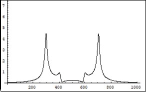
Download figure
Conclusions
The obtained numerical results allowed making the following conclusions:
1. The model of an elementary vacuum cell shows that a Quantum recurrence which represents the dynamics of virtual transformations in the cell, qualitatively differs from that of Poincare and the Fermi-Pasta-Ulam. Whereas these recurrences develop in time or space, the Quantum recurrence develops in a sequence of Fourier images represented by non exponentially separating functions. The sequence experiences random energy additions but no exponential separation occurs.
2. The Quantum recurrence can be defined as the most frequent array of Fourier images that appear in a certain quantum system during a period of its observation.
3. Different scenarios of the Fourier images sequences interpreted as bosons (electron and positron) and fermions (photons) apearing in the solutions of the model demonstrate that during some periods of its observation they become indistinguishable.
4. The quantum dynamics of every vacuum cell depends on the dynamics of many other vacuum cells interacting with it, thus the quasi periodicity (during the period of observation) of the Fourier images recurrence can have infinite periods of time and space and the amplitudes of the Fourier images can vary many orders in their magnitudes. Such recurrence times does not correspond even roughly to the Poincare recurrence time of an isolated macroscopic system. It reminds the behavior of spatially coupled standard mappings with different parameters.
The amount of energy in the physical vacuum is infinite but extracting a part of it and converting, it into a time-space form requires a process of periodical transfer of the reversible microscopic system dynamics into that of a macroscopic system. This process can be realized through a resonant interaction between the classical and quantum recurrences 12 developing in these two systems.
References
- 3.Largo E. (1998) The Fermi-Pasa-Ulam Problem revised. The Rockefeller University. , 1230 York Avenue, New York,USA 10021-6399.
- 4.Berezin A A. (2003) Modeling of coherent and stochastic properties of physical and biological systems. , (in Russian) Moscow
- 8.Feynman R P, Leighton R B, Sands M. (1963) The Feynman lectures on Physics. Vol. 8,9.QuantumMechanics.Addison-WesleyPublishingCompany
- 10.Berezin A A. (2004) Interaction between the FPU recurrences within the framework of coupled standard mappings. , Journal of Mathematical Modeling (Russia). v 16(8), 124-128.